Multiscalar Territorial Analysis User's Manual
| Revision History | |
|---|---|
| Revision 1.0.2 (svn rev 1088) | 2013-07-05 15:23:46 |
| Added some information about the "cities" layer over the maps. | |
Abstract
This document provides the minimum information about how to use ESPON HyperAtlas and ESPON HyperAdmin from the ESPON HyperCarte Web Application version 1.0.2.
Table of Contents
- Introduction
- 1. Overview
- I. ESPON HyperCarte Web Application
- II. ESPON HyperAtlas
- III. ESPON HyperAdmin
- A. Annex: when things go wrong...
- B. Annex: templates units names
- C. Annex: acronyms
- D. Annex: glossary
- E. Annex: references
- F. ESPON 2013 HyperAtlas Terms and Conditions of Use
- G. About
List of Figures
- 2.1. ESPON HyperAtlas License
- 2.2. Dataset Page
- 2.3. Log in Page
- 2.4. Help
- 3.1. Registered status menu bar
- 3.2. Advanced status menu bar
- 3.3. Hyps upload form
- 4.1. Security Warning
- 4.2. Security Warning: More Information
- 4.3. Security Warning: Certificate Details
- 6.1. ESPON HyperAtlas frame overview
- 6.2. Screenshot of the File menu
- 6.3. Screenshot of the View menu
- 6.4. Display submenu options: cities layer
- 6.5. Displayed cities
- 6.6. Screenshot of the Tools menu
- 6.7. Study area creation window
- 6.8. Study area creation success
- 6.9. Map of the new study area
- 6.10. Screenshot of the Session menu
- 6.11. Screenshot of the Help menu
- 7.1. Study area fields
- 7.2. Combination of study area and elementary zoning
- 7.3. Indicators box
- 7.4. Numerator, denominator and ratio tabs
- 7.5. Contexts box
- 7.6. Deviations maps tabs
- 7.7. Synthesis map options
- 7.8. Synthesis map tab
- 7.9. A deviations synthesis histogram for a regiion
- 7.10. Legend of the dual synthesis map
- 7.11. Dual synthesis map: red units
- 7.12. Dual synthesis map: blue units
- 7.13. Dual synthesis map: yellow units
- 7.14. Dual synthesis map: final typology
- 8.1. Details box for the synthesis map
- 8.2. Options for proportional circles
- 8.3. Options for deviation maps
- 8.4. Spatial zoom slider
- 8.5. Screenshot of a generated report
- 9.1. Expert mode enabled
- 9.2. Lorenz curve, statistical indexes and explanations
- 9.3. Equi-repartition map
- 9.4. Boxplots chart
- 9.5. Spatial autocorrelation chart
- 10.1. ESPON HyperCarte Workflow
- 11.1. First step: select a template
- 11.2. HyperAdmin templates list
- 11.3. EUROMED study area geometry template overview
- 11.4. EU 27 NUTS 2 study area geometry template overview
- 11.5. EU 27 NUTS 3 study area geometry template overview
- 11.6. EU 31 NUTS 2 study area geometry template overview
- 12.1. Step2: provide your data
- 12.2. Upload data page
- 13.1. Dataset information form
- 13.2. Successfull build
- A.1. Java console: stroke shape error
- D.1. Mathematical formula of the relative deviation
- D.2. Ratio
List of Tables
- 12.1. V2 sample About sheet
- 12.2. V2 sample Data sheet
- 12.3. V2 sample Default sheet
- 12.4. V2 sample Label sheet
- 12.5. V2 sample Metadata sheet
- 12.6. V2 sample Provider sheet
- 12.7. V2 sample RatioStock sheet
- 12.8. V2 sample StockInfo sheet
The next chapter, Overview, proposes an overview of a typical Multiscalar Territorial Analysis (MTA) session with ESPON HyperAtlas v2. Then, this document aims at providing an user's manual for the usage of the following applications:
![[Note]](../images/note.gif) | |
First of all, please insure that you have carefully read the ESPON 2013 HyperAtlas Terms and Conditions of Use. |
HyperCarte Research Group aims at providing projects and applications for interactive cartography. The projects focus on the development of an easily understood methodology that allows the analysis and visualization of spatial phenomena, taking into account its multiple possible representations.
Statistical observations of the territory are complex, and one representation, directly linked to a precise objective, is the result of a combination of different choices which are relative on one hand to the territories and their geographical scales, to the the statistical indicators on the other hand. This is of interest for researchers as well as for development policy decision-makers.
Thus, the principal innovative aspect of the HyperCarte project lies on this perspective based on the popularization of methods coming from spatial analysis such as the fitting of territorial scales, gradients, discontinuities…. This supposes an effort of multidisciplinary cooperation between geographers and computer scientists in order to create new maps in real time according to the different choices. An important effort has concerned ergonomics and time of calculus.
Main partners of the HyperCarte research group are:
| RIATE [UMS 2414] http://www.ums-riate.com | |
| CNRS UMR 8504 Géographie-Cités [UMR 8504] http://www.parisgeo.cnrs.fr | |
| LIG-MESCAL [UMR 5217] http://mescal.imag.fr/ | |
| LIG-STeamer [UMR 5217] http://steamer.imag.fr/ |
For more information, please visit HyperCarte Research Group Web site on http://hypercarte.imag.fr.
As an introduction, this chapter proposes an overview of a typical ESPON HyperAtlas v2 session, describing possible paths of investigation.
Users of the ESPON HyperAtlas v1 may remember the typical path of investigation, they were supposed to follow the seven following steps:
Choice of area, zoning and indicator of interest (that's to say a ratio)
Visualization of the ratio and (eventually) visualization of numerator and denominator without transformation
Analysis of inequalities at large level
Analysis of inequalities at medium level
Analysis of inequalities at local level
Synthesis of inequalities at large, medium and local level
Export of results towards a report
Of course, users are free to develop their own paths of investigation, and we can imagine different types of scenarios where users do not follow steps 1 to 7, but they adopt different strategies.
Let's now consider the following examples to demonstrate the benefits of a Multiscalar Territorial Analysis approach thanks to ESPON HyperAtlas:
Example 1
A stakeholder interested in the reform of structural funds after 2013 will probably use a path of investigation following the type (1)=>(3)=>(7) that will be repeated many times in order to test various scenario of allocation of funds. For example, what happens if:
NUTS2 is replaced by NUTS3?
GDP pps is replaced by GDP in Euro?
the threshold of 75% of EU mean is replaced by 80%?
Turkey joins EU?
etc.
Example 2
A local decision maker mainly interested in its region may use a path of investigation following the type (1)=>(6)=>(Save map), if the objective is to quickly extract three figures describing the situation of the regions at European, National and Local levels for a given criteria. He/she can then decide to click on other regions in order to benchmark its situation with neighbouring areas, or to identify other regions with the same strength and weaknesses. He/she can also decide to modify the indicator and to explore the strength of weaknesses of his/her region for various criteria, GDP/inh, unemployment, accessibility, ageing, etc.
Example 3
A spatial economist interested in economic convergence may decide to examine the situation of regions according to vertical contexts (e.g. belonging of region to a state, an INTERREG area) and horizontal contexts (e.g. difference between a region and its neighbours for different thresholds of contiguity or distance). He/she will therefore follow the expected steps (1) to (7), but he/she will probably introduce loops in the steps (4) and (5) in order to explore different variants of vertical and horizontal context. The loop (1)=>(5) will for example provide answer on question like the GDP/inh. Of course, the region of Budapest is greater than the neighbours for a distance of one hour by road, but what happens for a distance of two hours on a truck? Four hours? etc.
Having established that different users will not pay equal attention to the different functions offered by HyperAtlas, we can also suspect that expert users will expect more sophisticated functions than non-expert users, who will be on the contrary reluctant to enter into complex indicators or results.
Considering these different types of users, ESPON HyperAtlas v2 provides an expert mode (see ESPON HyperAtlas expert mode chapter), opened on request by the user (expert users or curious). In summary, the expert mode provides the following tools that complete the typical path of investigation:
Equi-repartition maps, one per context, for Large, Medium and Small (local) levels
Lorenz curve and statistical indexes (Gini index, Hoover index, coefficient of variation, ...)
Boxplots
Spatial autocorrelation chart
This part describes the main pages of the ESPON Web Application embedding the ESPON HyperAtlas and ESPON HyperAdmin applications.
| |
Some pages are only available to registered users, hence the following dedicated chapters:
|
Table of Contents
First access to the Web Application invites the user to read and accept the conditions and terms of use of the HyperAtlas, as shown on Figure 2.1.
| |
On following screenshots, the |
The links on the top right menu bar of the page provides the main topics that are available for this ESPON HyperCarte application:
HyperAtlas: when the user accepts the conditions of use (see Figure 2.1) , he/she can execute the ESPON HyperAtlas v2 applet. This applet allows then to perform a multiscalar territorial analysis on a default dataset (currently: Economy and Social Affairs). Please consult ESPON HyperAtlas part of this document for further information on how to use ESPON HyperAtlas.
Dataset: for further analysis, this page provides a list of available datasets that can be loaded by the ESPON HyperAtlas v2 (Figure 2.2).
Log in: as shown on Figure 2.3, this page provides a form for registered users who can log into the application in order to access advanced features. Registered users are invited to consult Registered users section.
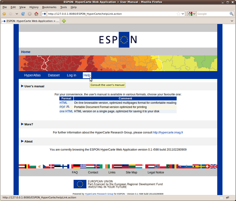
Help: displays links to the user's manual and the version of the Web Application, as shown on Figure 2.4.
Figure 2.1. ESPON HyperAtlas License
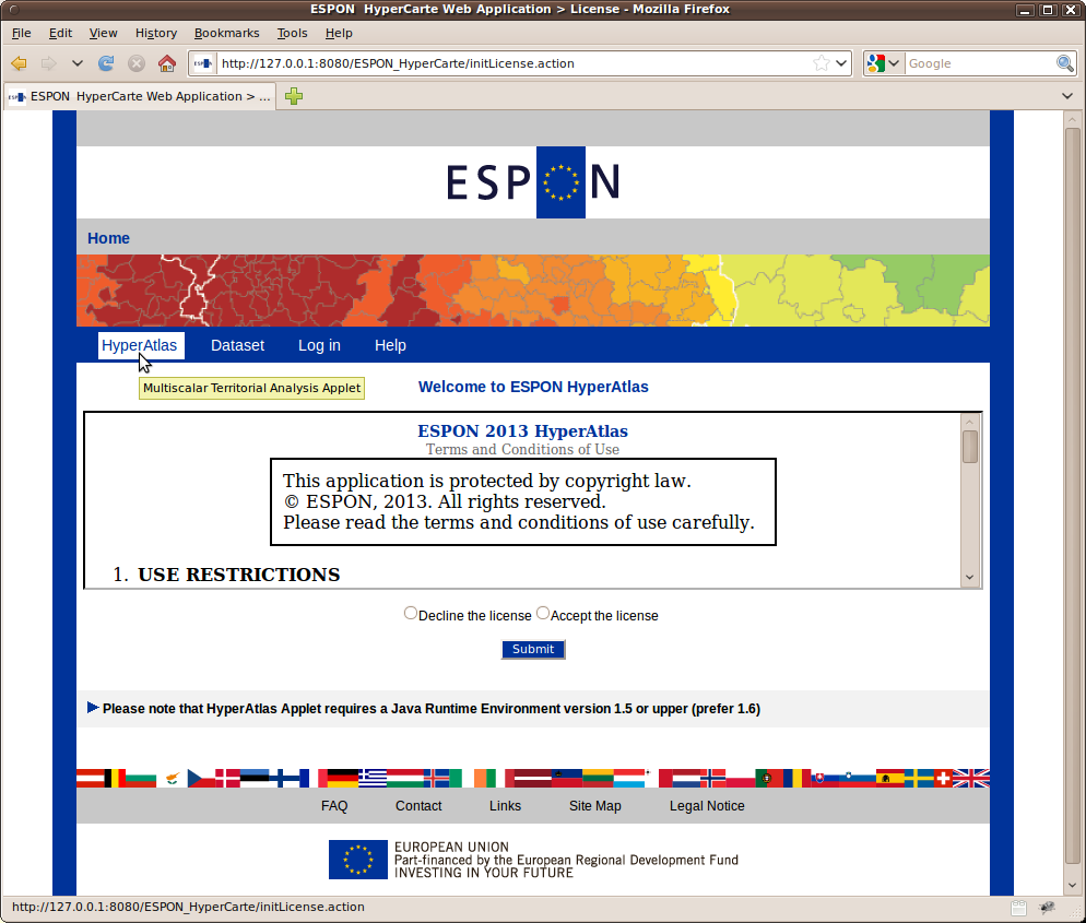
The license must be read and accepted by the user before accessing the ESPON HyperAtlas applet.
Figure 2.2. Dataset Page
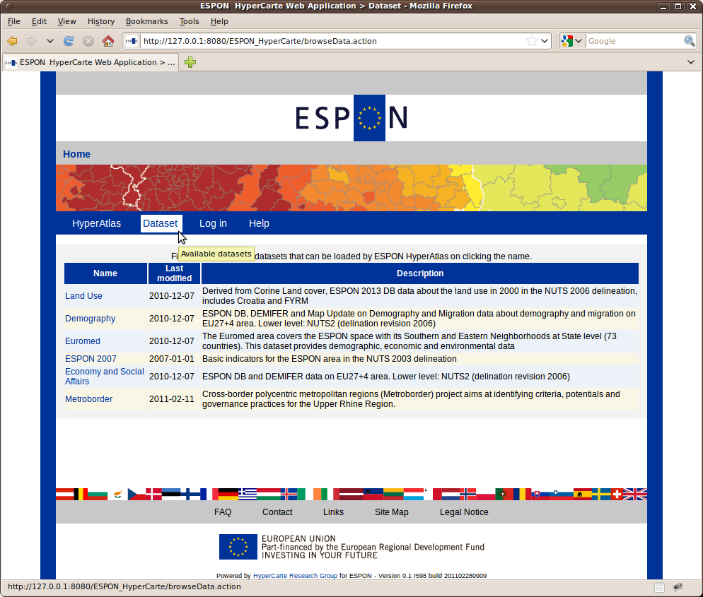
The list of available datasets on this page provides various thematics and study areas. Click the name of the dataset to load the associated hyp file into HyperAtlas.
Figure 2.3. Log in Page
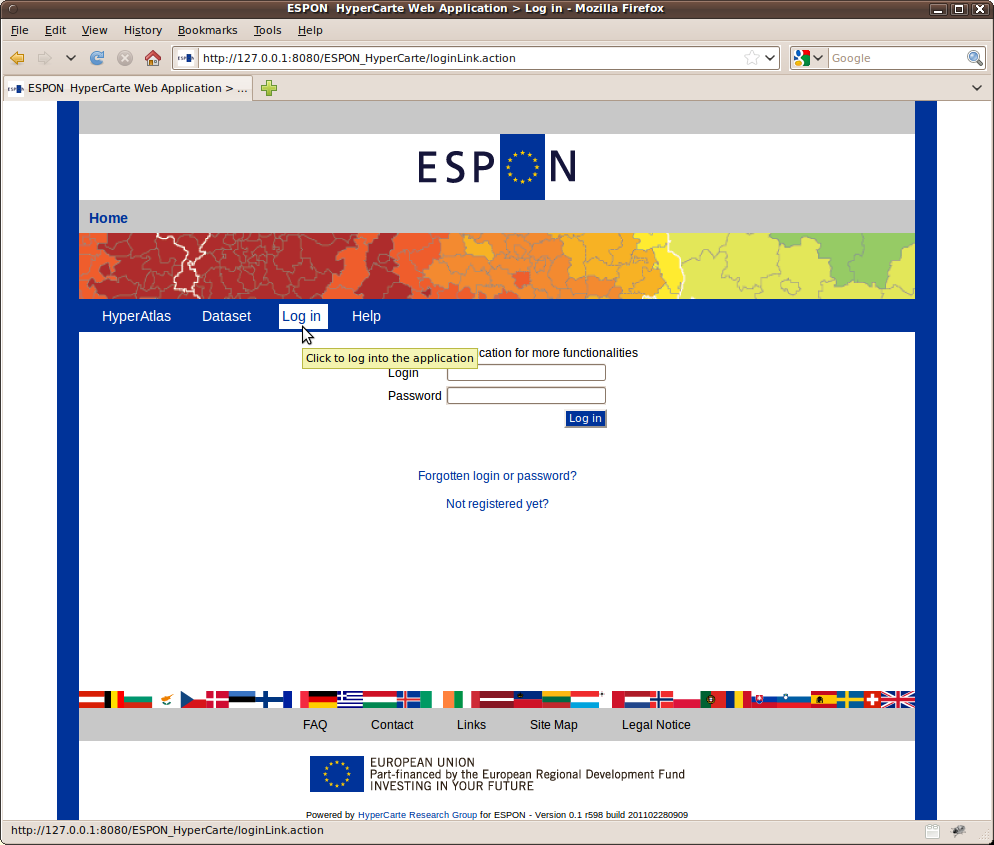
| |
"Forgotten login?" and "Not registered yet?" links are not implemented yet. Just check a "missing feature" page is returned on clicking these links. |
Once logged in with a valid login/password pair, available topics in the main menu bar of an authenticated session depend on the current user's status:
a user whose status is simply registered can use ESPON HyperAdmin integration tool to generate new dataset
.hypfiles.Figure 3.1. Registered status menu bar

The main menu bar of the Web application for an authenticated user whose status is "Registered".
a user whose status is advanced can not only use ESPON HyperAdmin but he/she can also submit new datasets (
.hypfiles) in order to make them available to everybody from the "Dataset" page of the application.Figure 3.2. Advanced status menu bar
The main menu bar of the Web application for an authenticated user whose status is "Advanced".
The tools of the authenticated session can be summarized as a typical scenario in three steps:
create a new dataset: as building a new dataset is quiet an advanced subject, the detailed use of ESPON HyperAdmin is further described in the ESPON HyperAdmin part of this document.
check your newly created dataset hyp file from ESPON HyperAtlas (see ESPON HyperAtlas part of this document)
submit the dataset ("advanced" status users only) as described below, How to submit new dataset hyp files?
The "hyp(s)" page of the authenticated session provides a form to upload an hyp file from your disk to the server, as shown on Figure 3.3. The form requires the input of a name and of a description for your dataset. This name and this description will be displayed in the table of the "Dataset" page (see Figure 2.2), they are independant of the name and description you have entered while creating this dataset.
Figure 3.3. Hyps upload form
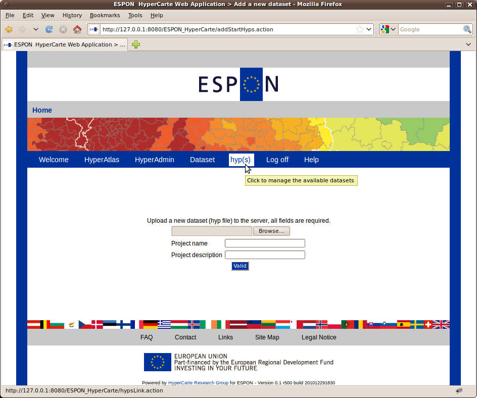
Requires an hyp file, a name and a description for the dataset to be added.
![[Important]](../images/important.gif) | |
Please test your |
ESPON HyperAtlas is a tool for Multiscalar Territorial Analysis: several indicators on the basis of the ratio of two initial geographical indexes can be derived, according to different spatial contexts.
Multiscalar Territorial Analysis is based on the assumption that it is not possible to evaluate the situation of a given territorial unit without taking into account its relative situation and localization. Regions belong to territorial and spatial systems. Indeed, from a policy point of view and in a social science perspective, contrasts and gradients are of much more interest than absolute values. Furthermore, aggregating and disaggregating territorial units allow to see how local values add up to form territorial contexts and regional positions.
Whatever the indexes used for political decisions, they have to be evaluated in relative terms. This may be done according to various territorial contexts. Thus one spatial organization may be examined from three different viewpoints that are three territorial contexts. They are differentiated according to the scale of political intervention or action they are referring to and that have a sense for the questioning: a global one, a medium one and finally a local one. Thus what is represented is the deviations to the three reference values associated to these different levels.
Let us take the example of the European union as a set of 25 countries, at the level of the region (NUTS2 for instance), and let the observed index be the wealth per resident in the regions (GDP/inh.). It is possible with ESPON HyperAtlas to consider the level of wealth of the regions relatively to three territorial contexts, and not only from an absolute point of view. The chosen contexts may be for instance respectively:
the whole European Union;
the country;
the neighborhood defined by contiguous regions.
ESPON HyperAtlas proposes for such an indicator a set of maps and charts that will be furthermore described in MTA parameters and Tools:
First maps show the selected study area, both the parent distributions as disc maps (here, wealth and population) and their ratios, that is to say the chosen index’s one.
Then, three maps show the relative deviations to the three chosen contexts as choropleth maps. For the above example: the deviation of a region to the European reference area, the deviation of a region to its national reference area, and in the third place the deviation of a region to the local reference area.
Then, two synthesis maps allow to evaluate the different combinations of the three previous relative deviation maps.
More advanced users are also provided a set of new tools like the maps of redistribution, the Lorenz curve and a chart of spatial autocorrelation.
| |
Here are some political justifications about the contextual and multilevel mapping, based on the European example:
|
| |
Before starting ESPON HyperAtlas: ESPON HyperAtlas is available on-line from the ESPON HyperCarte Web Application (see Figure 2.1 in All users chapter). Based on the Java technology applet, ESPON HyperAtlas requires a standard Web browser and a correctly installed Java Runtime Environment (JRE) plugin. This JRE is available by default on all standard Web browsers, whatever the platform is. A version 1.6 or upper of the JRE is advised, when available for your operating system. Nevertheless, on Mac OS X 32 bits platform, the user can currently (2010) not select a more advanced version than 1.5, but ESPON HyperAtlas is compatible with this version. So, please update your environment to get at least this version 1.5 of the JRE, but prefer the 1.6 when possible. For more information about your JRE, please consult the following links (last visit: 20101228): |
Before starting the application, the user is warned that the HyperAtlas Applet is about to be run without the security restrictions that are normally provided by Java.
Indeed, ESPON HyperAtlas is allowed to read-write on the user's disk to load a personal .hyp file or to write an html report for example.
To overcome the default behaviour of Java Applets that are not allowed to write on the user's disk, the ESPON HyperAtlas applet has been signed with a CNRS-2
standard certificate (CNRS is an acronym for Centre National de la Recherche Scientifique).
Thus, the security warning window (Figure 4.1) which is opened before the startup of the application is expected. The user can insure about the content he is about to execute by opening the details of the certificate, as shown on figures Figure 4.2 and Figure 4.3.
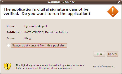
Figure 4.2. Security Warning: More Information
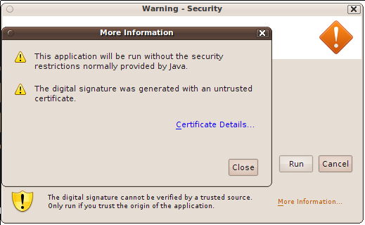
The user has clicked the More information... link on the bottom of the window Figure 4.1
Figure 4.3. Security Warning: Certificate Details
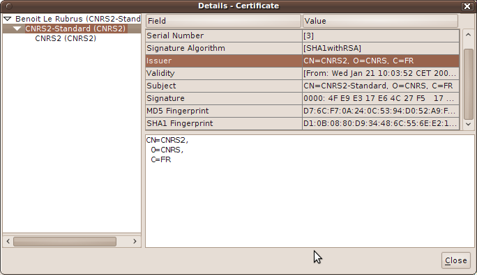
The user has clicked the Certificate details... link on the bottom of the window Figure 4.3
Once the user has clicked the Run button on the security warning popup window, the ESPON HyperAtlas applet begins to load a dataset. Depending on the speed of this loading, a splash screen icon may appear a few seconds:
The datasets provided by geographers are serialized in a convenient format for
ESPON HyperAtlas to a binary file named with the .hyp extension (example: Europe_2007.hyp).
As a convention, these ESPON HyperAtlas dataset input files will be now called hyp files.
| |
A complete description of the ESPON HyperAtlas integration tool, named ESPON HyperAdmin, is available from the ESPON HyperAdmin part of this document. |
ESPON HyperAtlas is designed so it can load any dataset serialized as an hyp file.
From the "HyperAtlas" menu item of the HyperCarte Web Application main menu bar, once the user has accepted
the terms and conditions of use (see Figure 2.1), the ESPON HyperAtlas
loads a default dataset: Economy and Social Affairs.
The user can also load a dataset hyp file from his disk via the "File-Open" menu item of the application.
Customized datasets for various topics are also available from the "Datasets" page of the Web Application, see Figure 2.2.
ESPON HyperAtlas is totally interactive. It works with three sets of parameters that are linked to one or more maps. At any time, the user can change the different input parameters, and the linked maps are immediately updated. The user may also individually configure each map, for instance:
the number of equivalence classes
statistical progression (arithmetic or geometric)
the pallet of colors
etc.
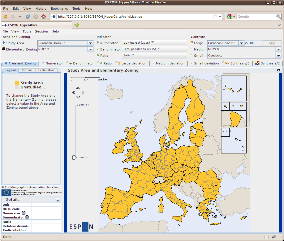
As shown on Figure 6.1, ESPONHyperAtlas Applet fills the full width of the browser window. A "Back to dataset" link at the top of the page allows the user to be redirected to the ESPON HyperCarte Web Application "Dataset" page. The main components of the ESPON HyperAtlas frame are:
a menu bar
the parameters panel threefold boxes:
Area and Zoning to select the geometric parameters of the analysis;
Indicator to select stocks or pre-defined ratios;
Contexts for the deviations to select the references of computed deviations.
a main panel composed of the generated maps
Following sections first detail each item in the menu bar of the application.
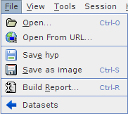
This menu allows:
to open a new dataset
hypfile from your disk or from an eventual known URL (Unified Resource Locator) to anhypfile located at a server on the Internet;to save the current dataset to your disk as an
hypfile;to save the current displayed tab as an image (PNG) file to your disk;
to generate a report in HTML format, including an image each current tab of the current analysis.
to be redirected to the Web Application Dataset page in order to load another on-line dataset (see Figure 2.2)
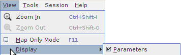
This menu concerns the appearance of the maps. It provides menu items to zoom in, zoom out and to choose the different panels that can be displayed as different parts of the window:
the "Map only mode - F11" allows to display the map frameset as wide and high as possible;
the "Display - Parameters" menu item makes the parameters panel visible or note.
Depending on the current loaded dataset, the "Display" submenu may also include an additional checkbox item as shown on the Figure 6.4. This checkbox allows the user to display or hide the main cities over the map. By default, if the dataset provides such a layer, it is checked.
Figure 6.4. Display submenu options: cities layer
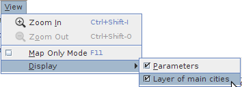
On this screenshot, the loaded dataset embeds the main cities. The "Display" menu allows to hide or display this additional layer.
When the Display-Cities menu item is enabled, cities are displayed over the maps as black squares, as shown on Figure 6.5. Note that for ergonomy reasons, to avoid overlapping between cities labels, the names of the cities are not displayed over the map. Nevertheless, a tooltip appears when the mouse comes over a square.
Figure 6.5. Displayed cities
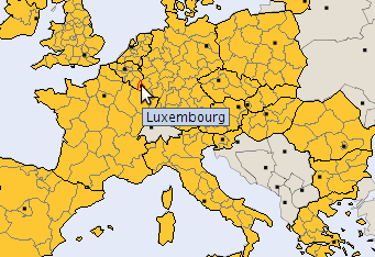
Cities are represented as black squares. The name of the city appears when the mouse moves over a square.
The Popup Freeze menu item has been available since HyperAtlas v2. This functionnalitiy is usefull to compare several maps or charts: clicking on this menu item, a popup window is opened, displaying a frozen image of the current visisted tab.
Two options allow to manage the behavious of the mouse cursor:
The Turn Pan menu item allows to enable the moves of the maps inside the window.
The Turn Histogram menu item is only enabled for the synthesis map, it displays for each region the three contextual deviations (see synthesis as an histogram paragraph)
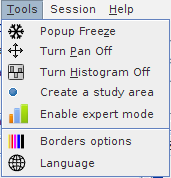
Other tools available on this menu:
Create a study area menu item is described below.
Enable expert mode" menu item is described in ESPON HyperAtlas expert mode chapter of this document.
Borders options: use this item to choose the colors of borders of territorial units for example.
Language: this menu item opens a dialog box that provides the list of available languages for the interface of the frame. The internationalization feature is currently available in english, french and romanian. The default language at startup depends on the locale of your system, english by default.
This version 2 of ESPON HyperAtlas allows to define a new study area. On clicking this menu item, the user is invited to enter a name for his/her new study area and to select the top-levels units (as a rule, countries) that will compose this study area.
Figure 6.7 shows the example of a user who wants to define the benelux study area.
He/she selects Belgium, Luxembourg and Nederlands units then clicks the "Submit" button.
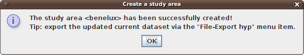
Figure 6.8 shows the information message that is displayed when the creation is successfull. The benelux
parameter is now available from the Study Area combo box of the parameters panel.
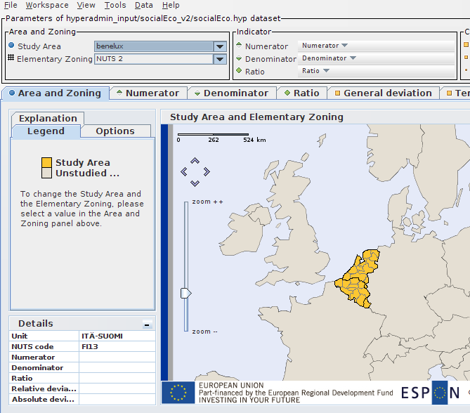
Figure 6.9 shows that interactive maps have been consequently updated on selecting this new study area.
Figure 6.7. Study area creation window
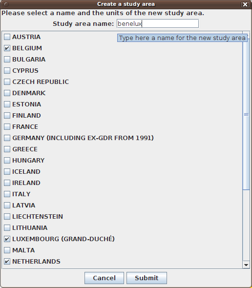
Provides the list of countries and a text field to enter a name for this new study area.
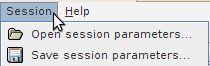
This menu allows to save the parameters of the current analysis to an ESPON HyperAtlas XML file on your disk.
In the case when you already saved such a file, this menu allows to load your previous session parameters.
| |
A session parameters file is specific to a dataset. An error occurres if you try to load a session parameters file that was built while using another dataset. |
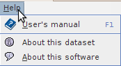
This menu provides the following items:
Help (F1): opens a new browser window to the on-line user's manual (see Figure 2.4).
About dataset opens a popup window displaying metadata of the current dataset (author, creation date, version).
About displays the current version of the software. Please note this version when reporting an eventual bug as described in Annex: when things go wrong.
Table of Contents
This section focuses on how to set the parameters for a Multiscalar Territorial Analysis (MTA). As its title suggests it, the next section (An example of multiscalar typologies of regions) first describes the main concept of such an analysis. Please read it in order to efficiently benefit of the provided tools by ESPON HyperAtlas v2.
| |
Some screenshots of this chapter were performed with a previous version of HyperAtlas. Though the graphical user interface has been updated since this version, the concepts remain the same. |
Taking account the European level as an example, this section focuses on the importance of considering the multiscalar typologies of regions in political decisions.
When the policymakers want to build political scenari or when they want to evaluate propositions of structural funds, they need to get a synthetic view on the situations of regions which depend on the various territorial contexts.
The question of perequation (transfer from “advanced” to “lagging” region) is very sensible and it is important to propose a complete view of the scales where those perequation processes can take place, according to the principle of subsidiary.
As an example, we analyse how the picture of “lagging” regions is modified when the previous criterion of Objective 1 (less than 75% of the mean value of GDP) is applied simultaneously at three scales: European, national and local.
Simultaneously, it is possible to propose a typology of “advanced regions” based on the symmetric criteria of more than 133% of the mean value of GDP at those three scales.
According to this methodology, it is possible to demonstrate that very few regions are “lagging at all scales” and “advanced at all scales”. Many are in more complex situations, like certain regions of Switzerland or Norway which are “advanced” at European scale, but they are “lagging” at their national or local scales.
Reversely, the metropolitan regions of candidate countries are very often “lagging at European scale” but “advanced at national and local scales”.
The setting of the study area should be the first step of any analysis. Setting the basis of the study can be done by answering the following questions:
which spatial extension (area) and for which geographical level?
which division will be the elementary zoning?
Figure 7.1. Study area fields
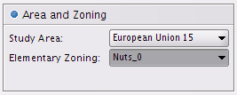
Study Area shows the spatial extension that will be mapped.
Elementary zoning shows the set of elementary units that will be studied.
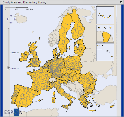
Figure 7.2 illustrates two possible combinations. The selected area is mapped when the chosen elementary zoning is drawn.
Figure 7.2. Combination of study area and elementary zoning
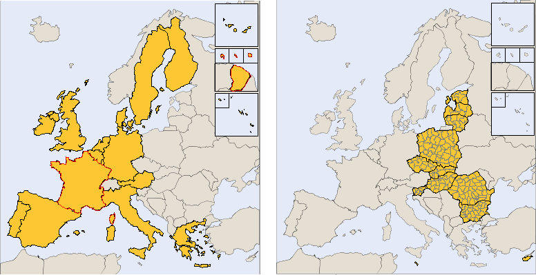
These two maps were extracted from the "Area and Zoning" tab of the application with following settings:
| Study Area | Elementary Zoning | |
|---|---|---|
| Map on the left | European Union 15 | NUTS 0 |
| Map on the right | New member states 12 | NUTS 3 |
ESPON HyperAtlas only works with size variables (that is to say that only variables that may be aggregated at upper level by sum), and proposes a multiscalar cartography of the ratio for two size variables in order to set the studied ratio. The user can combine every couple of these types of variables in the “Indicators” box, by choosing each of them in the associated select boxes as shown on Figure 7.3.
Figure 7.3. Indicators box
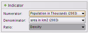
This box provides three select boxes to choose indicators. The user selected the Density item in the Ratio
select box:
Numerator is set to
Population in 2003Denominator is set to
Area in km2Ratio: depending on the chosen dataset (the hyp file), selecting a ratio may implie the auto-selection of the numerator and denominator fields values.
Three maps are respectively linked to these choices, under three different tabs (see Figure 7.4). The maps for the numerator and for the denominator (size variables) are represented with proportional circles. The ratio map is shown with colored units, according to the ratio value. The number of classes and their associated colors (the pallet tool) can be can be set in the "Option" tab of the ratio map.
Figure 7.4. Numerator, denominator and ratio tabs
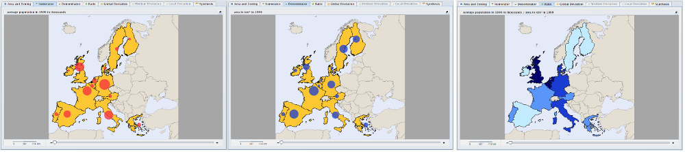
The three associated tabs to the chosen indicators are represented here for the study area EU 15 (15 countries in Europe)
with the NUTS 0 value (countries) for the elemetary zoning:
the image on the left shows the Numerator map within its associated tab, here, the
population in 2003the image in the center shows the Denominator map within its associated tab, here, the
area in km2the image on the right shows the Ratio map within its associated tab, here, the density.
As described in various contexts paragraph, the user has to define the three territorial contexts which respectively set three different levels of spatial observation: global, medium and local. Figure 7.5 shows the select boxes to set these parameters.
![[Caution]](../images/caution.gif) | |
The names of the references have been updated since the previous versions of ESPON HyperAtlas:
|
Figure 7.5. Contexts box
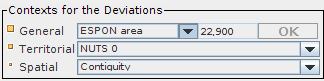
The "Contexts" box allows to set three references for their associated deviations: general, territorial and spatial contexts.
The general context may be the whole chosen study area. In such a case, the associated map will be the same as the associated map to the ratio itself. So, the user may choose another general context or a reference value. For instance, in the example of the EU, even if the study area is the 29 potential countries, it may be of interest to observe the spatial differentiations according to another global reference, for instance the global value associated to EU15. For this level, the user may also exogenously enter a value. By default, this value has first been set to the value of the global area.
The territorial context, on the other hand, has to be a geographical zoning that is an aggregation of the “elementary zoning” that was previously chosen.
The spatial context shows which proximity relation will be the basis of the neighborhood’s definition for each elementary unit. That is usually “contiguity”, but it may also be a relationship based on distances since they have been introduced in the hyp file (units that are less than X kilometers far from), or time-distances. Then, each elementary unit value will be compared to the value of its neighborhood.
A set of three maps are linked to these choices (Figure 7.6). The values of the deviations are transformed into global indexes 100. Thus, values may be interpreted in terms of percentage to the reference value. The maps are drawn with double progression frame centered on 100, in order to highlight the regions that are under the reference value (100), and the ones that have upper values.
Figure 7.6. Deviations maps tabs
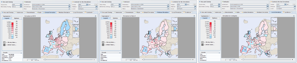
These screenshots show the three deviations maps tabs for chosen contexts: general deviation on the left, territorial deviation in the center and spatial deviation on the right.
One synthesis map was already available in the previous version of ESPON HyperAtlas, based on three levels and one treshold, it is described in Ternary synthesis map. A new synthesis map has been added to the application since the version 2.0: see Dual synthesis map.
The three relative positions about contexts are summarized in one synthetic map. The elementary units are classified in eight classes according to their three relative positions.
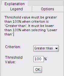
In order to reduce the whole combinatory of possible cases, from the "Options" tab close to the synthesis map (Figure 7.7), the user must specify which point of view he wants to focus on: the first "Criterion" parameter shows whether the point of view is to underline the regions whose ratio is greater than, or to underline the contextual values, by selecting less than. This choice depends on the studied indicator (see An example of multiscalar typologies of regions section). For instance high values of unemployment rates point out different types of regions than high values of an indicator of resources. According to which regions have to be differentiated (lagging ones or wining ones), the user must chosse the point of view of the synthesis. Then, the user can choose the threshold percentage.
The map on Figure 7.8 illustrates the eight different configurations of relative position, according to the three previously chosen contexts and parameters. The legend tab gives for each class the descriptions of the contextual positions. The last class (in white) gather the regions that are not concerned by the chosen comparative criterion whatever the contexts are.
Figure 7.8. Synthesis map tab
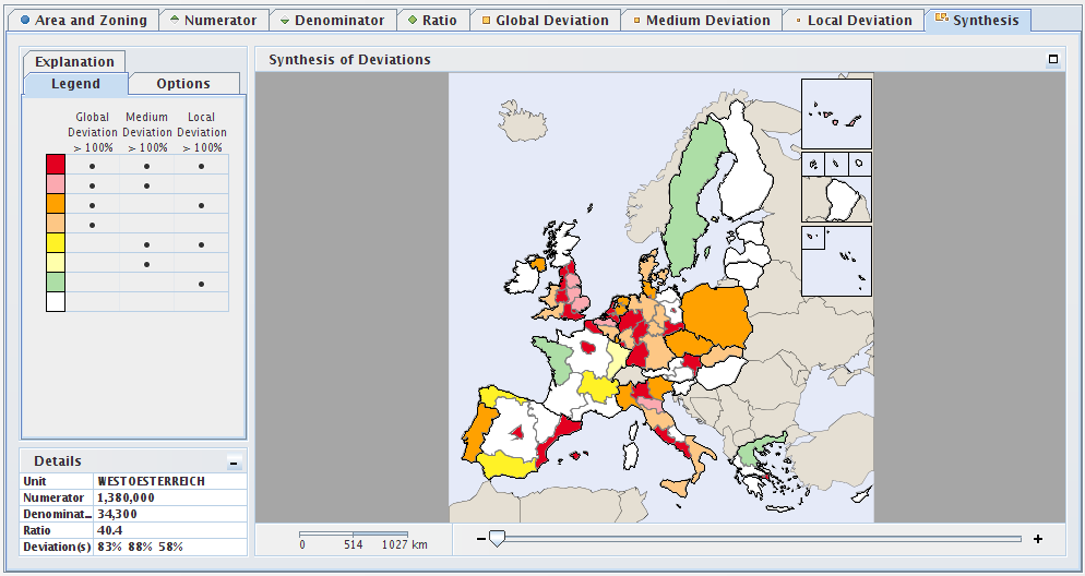
This screenshot shows the synthesis map tab for the contexts that were chosen in the previous example shown on Figure 7.6.
When “Histogram” is enabled (see Section 6.3 section), the user may represent the three contextual deviations of a selected (clicked) region as an histogram as shown on Figure 7.9.
Figure 7.9. A deviations synthesis histogram for a regiion
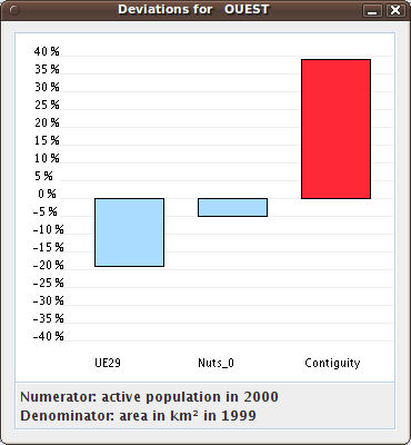
This screenshot shows the synthesis histogram of the clicked region named OUEST (West of France). The general deviation
of this region is relative to the UE29 general context. The territorial deviation is relative to the NUTS 0 hierarchical
context, the spatial deviation considers the contiguity, e.g. the neighborhood of this region.
The dual synthesis map is a new cartographic tool that has been introduced in the version 2.0 of ESPON HyperAtlas. It aims at showing via a chromatic legend the status of territorial units on taking into account two chosen deviations. This section describes the synthetis opportunity that is offered to analysts thanks to this tool.
The legend of the dual synthesis map shown on Figure 7.10 is composed of four main quarters. The values on both axis range range from 0 to 200% and they represent the percentages of a deviation of a territorial unit relatively to a context of reference. The user is invited to select in an options tab the contexts of deviations to be considered for both axis (among the general, the territorial or the spatial context).
Let's consider the following example: the general deviation has been chosen for the horizontal axis and the spatial deviation for the vertical axis. The four main colors of the legend represent the following cases:
yellow: the global deviation (X axis) is lower than 100% (the average pivot value) and the spatial deviation (Y axis) is upper 100%
red: both deviations are upper 100%
blue: both deviations are lower than 100%
green: the global deviation (X axis) is upper than 100% and the spatial deviation is lower than 100%
Figure 7.10. Legend of the dual synthesis map
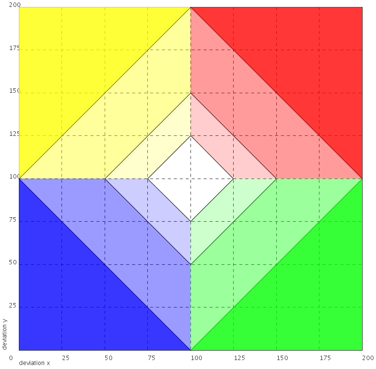
Graduations and quarters of the dual deviation synthesis map legend.
Let's consider now a concrete example on how the dual deviation map can help analysts: the following screenshots decompose as four steps the synthesis about the situation in 2010 according to the European and National averages of unemployement:
Figure 7.11 shows in red the territorial units whose unemployement rate is above average both at European and National levels:
Figure 7.12 shows in blue the territorial units whose unemployement rate is under average both at European and National levels:
Figure 7.13 shows in yellow the territorial units whose unemployement rate is above average at European level and under at National level:
Figure 7.14 shows the final typology on the complete synthesis map:
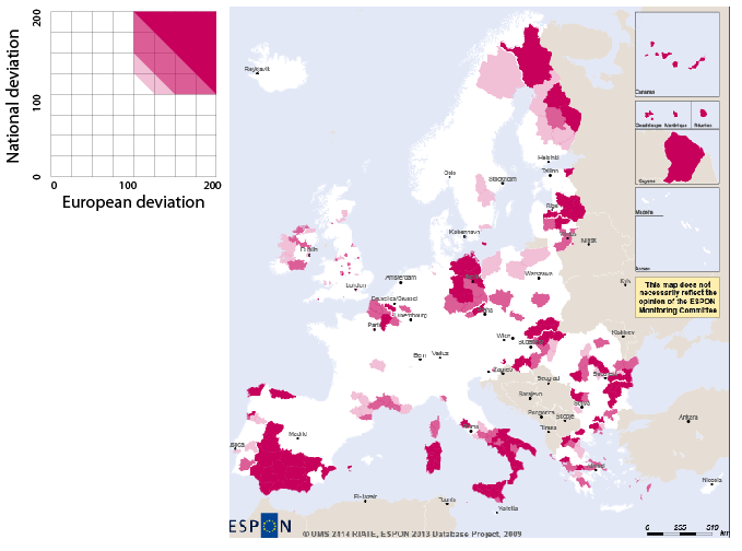
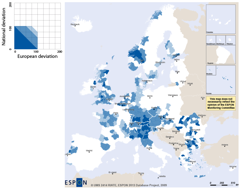
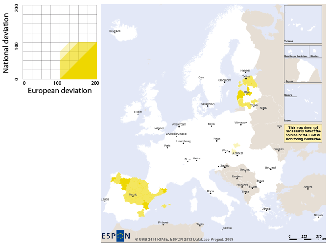
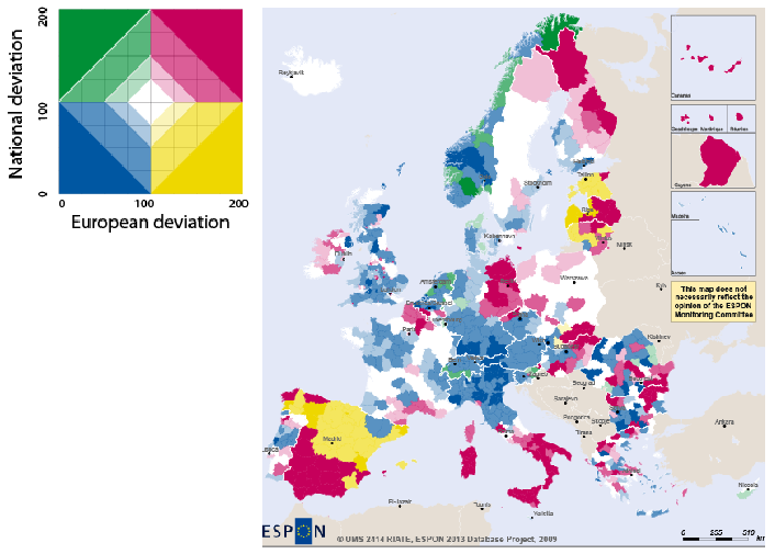
Table of Contents
This section deals with the available tools in the application to work with the maps.
First of all, let's review the available maps tabs and their main focuses:
 Area and zoning
This map shows the chosen study area and elementary zoning.
 Numerator
This map shows the chosen study area and elementary zoning.
 Denominator
This map shows the value of the chosen denominator indicator for each unit of the elementary zoning.
 Ratio
RatioThis map shows the distribution of the ratio (numerator/denominator) over the units of the elementary zoning.
 General deviation
This map proposes the relative perspective of the distribution of the ratio over the units of the elementary zoning: each absolute measure is put in relation with a reference value. The reference value is common for the whole area. The index value is 100 when an elementary unit has exactly the same value than the reference value or area. It is 200 when the elementary unit measure is twice the measure of the reference area, it is 50 when this is half the measure of the reference area.
 Territorial deviation
This map proposes the relative perspective of the distribution of the ratio over the units of the elementary zoning: each absolute measure is put in relation with the value of its upper unit in the reference zoning. The index value is 100 when an elementary unit has exactly the same value than its reference unit. It is 200 when the elementary unit measure is twice the measure of the reference unit, it is 50 when it is half the measure of the reference unit.
 Spatial deviation
This map proposes the relative perspective of the distribution of the ratio over the units of the elementary zoning: each absolute measure is put in relation with the value of its neighborhood, as defined by the local reference. The index value is 100 when an elementary unit has exactly the same value than its neighborhood. It is 200 when the elementary unit measure is twice the measure of its neighborhood, it is 50 when it is half the measure of its neighborhood.
 Synthesis
This map proposes a synthesis of the different perspectives by considering the three different contexts. The synthesis is based on a deviation threshold, either by upper values or by lower value. These parameters depend on the meaning of the ration and they must be chosen by the user. Then, a typology of the regions which check the condition for at least one context is performed.
 At any moment, the position of the mouse cursor on the map provides information
about the elementary unit that it points. The content of the table depends on the current map, Figure 8.1 shows
the case of the synthesis map where are displayed:
At any moment, the position of the mouse cursor on the map provides information
about the elementary unit that it points. The content of the table depends on the current map, Figure 8.1 shows
the case of the synthesis map where are displayed:
the name of the territorial unit
the code of this unit
numerator stock value
denominator stock value
ratio (numerator/denominator) value
relative deviations values based on the selected references
the absolute deviation values are only available in expert mode
Figure 8.1. Details box for the synthesis map
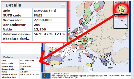
This screenshot shows the "Details" box on the left bottom corner of the application. The user's mouse is over the Guyane. Associated computed values to this unit are displayed in the box.
 Except for the synthesis map, a left click anywhere on the map changes the
function of the cursor to “Pan”, as long as this option is on (see Section 6.3).
Except for the synthesis map, a left click anywhere on the map changes the
function of the cursor to “Pan”, as long as this option is on (see Section 6.3).
 On the synthesis map, the "hand" mouse pointer shows that the
histogram function is on. A right click on a region opens its histogram synthesis view (see synthesis as an histogram).
On the synthesis map, the "hand" mouse pointer shows that the
histogram function is on. A right click on a region opens its histogram synthesis view (see synthesis as an histogram).
Each map is associated to a set of three tabs that provide tools to control and to understand the cartography. The choices are valid for the current map. Figure 8.2 displays each the "Options" tabs for an indicator map (that shows proportional circles) while Figure 8.3 displays the available options on a deviation map (palett of colors). The user may also set the thresholds for each class. The "Legend" tab displays the bounds of the classes (left), the number of items for each of them (right), and the associated color. The "Explanation" tab displays some general notes about the goal of the current map.
Figure 8.2. Options for proportional circles
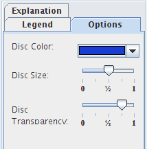
The "Options" tab of the numerator or denominator maps aims at setting the representation of the indicator values by selecting a color, the size and transparency of proportional circles.
Figure 8.3. Options for deviation maps
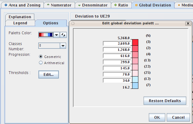
The "Options" tab of the deviation maps aims at setting the representation of the deviation by selecting:
the palett of colors, that can be reversed
the number of classes, between two and ten classes
the progression:
arithmetic for classes with an equal amplitude, better choice when the distribution is symmetric around 100.
geometric for classes with an increasing amplitude
the thresholds, that can be edited for each class
It is possible to zoom in/out a map, either on clicking the "View - Zoom" menu items, by using the cursor on the left side of the map or by moving the mouse scroller over the map.
| |
Please note:
|
Figure 8.4. Spatial zoom slider
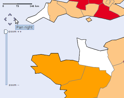
This screenshot shows the scale, the pan buttons and the zoom slider.
The user can save his current whole collection of maps with the associated rough data and deviations by selecting the "File - Build Report" menu item from the menu bar.
By selecting this menu item, the user is invited to select a directory on his/her disk where the report will be generated as a set of HTML page (index.html
and eight PNG image files (one image per map: map0.png, map1.png, to map7.png).
For example, if the user selected his /home/toto/my_hyperatlas_report/ directory as target directory, he/she may open the saved report from a web browser
by selecting the /home/toto/my_hyperatlas_report/index.html file.
The generated report may be divided in the three-fold:
the introduction shows the space area, chosen indicators and contexts
the list of maps for these parameters as images files
the table of generated results for these parameters
| |
In expert mode, the generated report also includes expert tabs as images:
|
Figure 8.5. Screenshot of a generated report
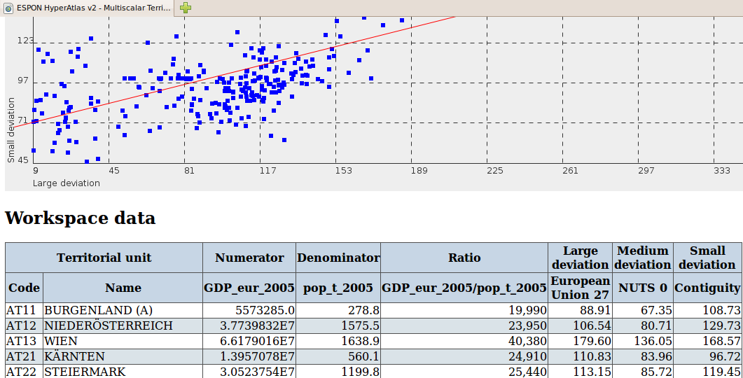
This screenshot shows an extract of the generated report index.html file that has been opened by in web browser.
This image shows the last map (synthesis) and the start of the table that includes all results.
Table of Contents
This chapter describes a set of tools that have been integrated since the version 2 of ESPON HyperAtlas. As this set of cartographic and statistic tools are mainly designed for more advanced users, they are not available by default at the startup of the application. In order to keep the application easy to use for not so advanced users, this set of tools must be enabled on clicking the Enable expert mode menu item of the "Tools" menu, shown on Figure 6.6.
Graphically speaking, enabling the expert mode adds six new tabs to the eight available tabs in default standard mode:
three tabs for equi-repartition maps (respectively for large/medium/small contexts of reference), they are described in Section 9.2 section.
a tab showing a Lorenz curve and a table computing relevant statistical indexes. This feature is described in Section 9.1 section.
a tab showing a chart of boxplots, described in Section 9.3 section.
a tab showing a spatial autocorrelation chart, described in Section 9.4 section.
In order to distinguish the default mode tabs and the expert mode tabs, expert tools tabs titles backgrounds are displayed with a golden colour. Enabling the expert mode automatically enables and displays the "equi-repartition" map for the large context, the list of tabs is shown on Figure 9.1.
Figure 9.1. Expert mode enabled

Default mode set of tabs is added six new tabs when enabling the expert mode.
| |
Depending on the operating system, the Java Runtime Environment version (1.5 or upper is required) and the user's browser, the display may differ. For example, under the Mac OS X.5 operating system with a JRE 1.5, the tabs are embedded in a scrollable list. |
The map of large deviation provided by ESPON HyperAtlas is a general measure of disparities for a given variable Z which is the ratio between two stocks X and Y. This estimation of general disparities can be further analysed using various econometric indexes that have been added in ESPON HyperAtlas v2 expert mode:
the Lorenz curve typically presents the cumulative proportion of population and resource when starting from regions with lowest resource per inhabitant.
the Gini Coefficient is a summary of the Lorenz curve measuring the global amount of disparities: it is equal to the area located between the Lorenz Curve and the diagonal (perfect-equality)..
the Hoover index, also called Disparity index, is another summary of the Lorenz Curve, as it is equal to the maximum distance between Lorenz Curve and diagonale.
The Coefficient of Variation is simply equal to the ratio between standard deviation and average of the considered ratio Z.
| |
A complete description of the Lorenz curve and of the main statistical indexes is directly available in a dedicated "Explanation" panel of the statistical box, close to the curve panel, as shown on Figure 9.2. |
Figure 9.2. Lorenz curve, statistical indexes and explanations
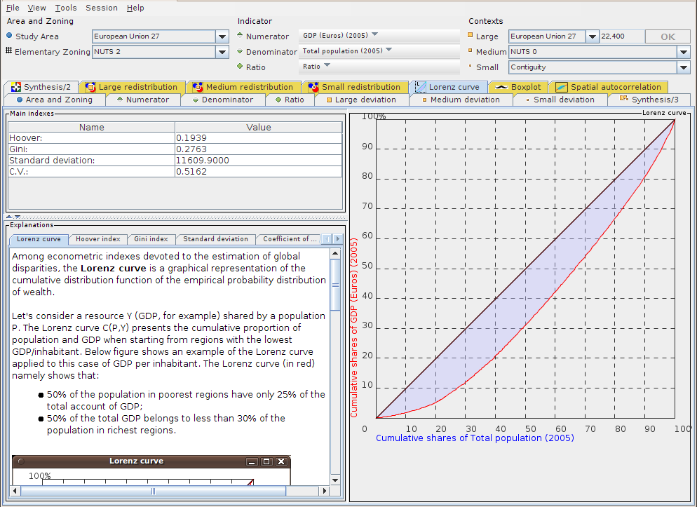
This tab shows the Lorenz curve, a table of main statistical indexes, and an "Explanations" titled panel providing some information for each feature.
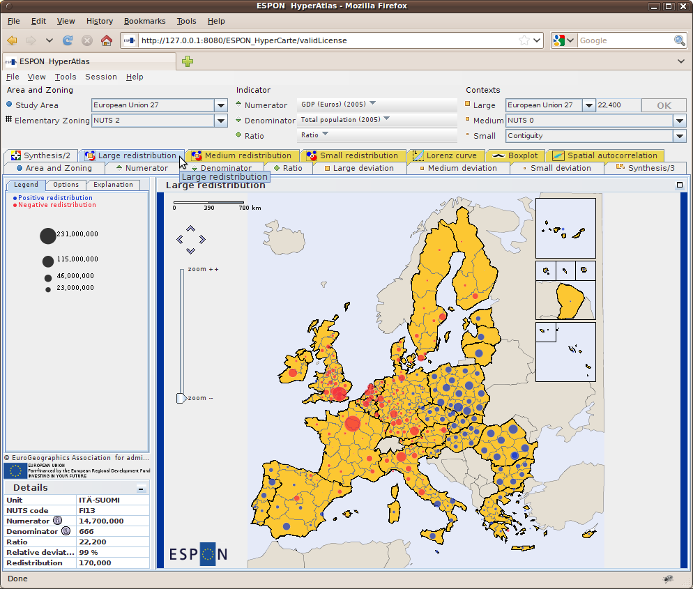
The equi-repartition maps indicate which process of redistribution should be realized in absolute terms in order to achieve convergence, at European, national or local levels.
The equirepartition map is a bi-color discs map showing an absolute deviation. It examines how much amount of the numerator should be moved in order to reach equi-repartition, for each territorial unit, taking into account as a reference the selected deviation context value.
Thus, three equi-repartition maps are available in expert mode for respectively the large, medium and local deviations tabs. As an example, Figure 9.3 shows the equi-repartition map (also called "Redistribution" map) for the large context.
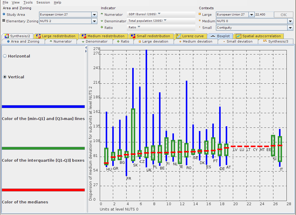
For each unit in the chosen medium context (NUTS 0 for example in Figure 9.4), this chart shows the dispersion of the medium deviation for the territorial units at sub-levels (NUTS 2 level in Figure 9.4).
A boxplot typically provides the following information:
two lines show the values between:
the minimum and first quarter Q1
the third quarter and maximum Q3
a box shows the interquartile Q1-Q3
a line shows the mediane value
The spatial autocorrelation chart is only available when the expert mode is enabled.
For each territorial unit of the study area, this chart crosses the values of the spatial deviation on absissa axis with the values of the territorial deviation on ordinates axis.
This chart is very interesting for expert users as it reveals spatial dependancy, e.g. spatial organization of a phenomena.
More empirically, the chart can also be used to examine the situation of outliers and exceptional units out of the cloud of points.
The compute of this chart is based on a Moran's coefficient of spatial autocorrelation variant. The regression line is drawn in red on the chart, its equation, computed by the least squares method, is displayed on the left corner of the frame, as shown on Figure 9.5.
Each unit is drawn as a blue square, its name is displayed in a tooltip when the mouse comes over the square.
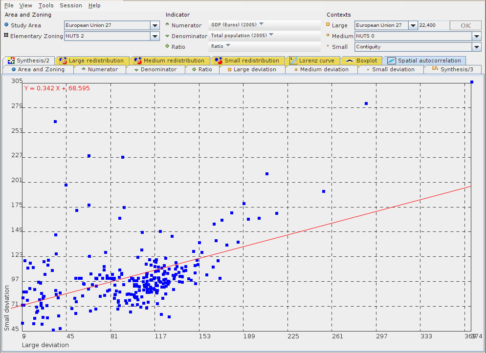
Table of Contents
In order to perform Multiscalar Territorial Analysis with ESPON HyperAtlas, the datasets provided by geographers are serialized in a convenient format
into a binary file named with the .hyp extension. As a convention, a ESPON HyperAtlas dataset input file is called an hyp file (example: demography.hyp).
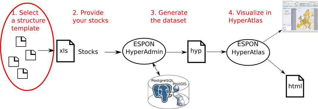
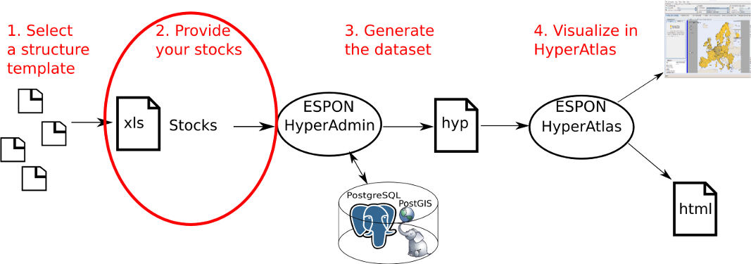
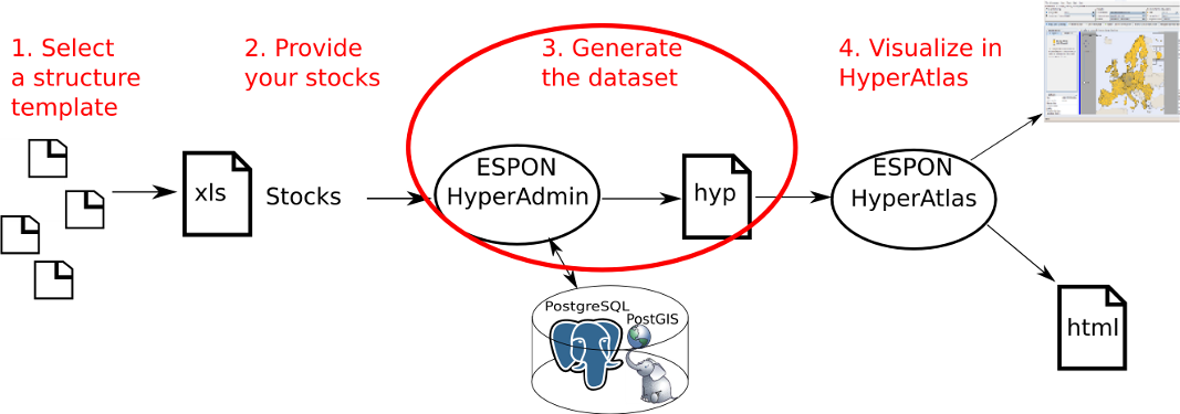
ESPON HyperAdmin is the tool to generate hyp files from your a set of input well-formed files. The steps to generate an hyp file and the workflow between ESPON HyperAdmin and ESPON HyperAtlas is summarized in the Figure 10.1.
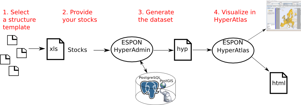
As shown on Figure 10.1, creating a dataset hyp file consists in:
preparing your dataset geometry as a MIF/MID files pair (MapInfo format);
preparing your dataset structure as a speadsheet
structure.xlsfile;optionally, preparing a distance-time matrix as an
xlsfile for custom contiguities;preparing your dataset stocks as a spreadsheet (Excel/OpenOffice)
data.xlsfile;generating the dataset
hypfile with ESPON HyperAdmin.
Following chapters describe each above step for integrating your data into an hyp file.
When starting the creation of a new dataset with ESPON HyperAdmin, the user is first invited to choose the model of structure on which he/she wants to add stocks.
As shown on Figure 11.2, the choice simply consists in clicking the name of the template among the ones that are listed and described in the table of this page.
Figure 11.2. HyperAdmin templates list
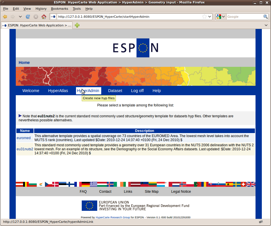
The table lists the available templates of structure/geometry ESPON HyperAdmin input. Note that all available templates are not listed on this screenshot, see below.
Find below a description of each available template:
euromed: this template considers the WUTS at ranks 3-4-5 (countries) delineations on the EUROMED area, as shown on Figure 11.3.
Figure 11.3. EUROMED study area geometry template overview
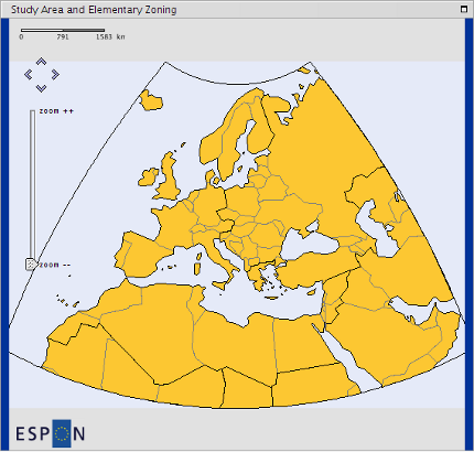
Delineation of the EUROMED geometry template at WUTS 5.
eu27nuts2: this template considers 27 European states, the delineation is based on the NUTS 2006 revision, at NUTS 2 lowest mesh level. The Figure 11.4 provides a screenshot of the maximal available study area:
Figure 11.4. EU 27 NUTS 2 study area geometry template overview
Delineation of the EU 27 NUTS 2 geometry template.
eu27nuts3: similar to previous template, but the lowest mesh level considers NUTS 3. The Figure 11.5 provides a screenshot of the maximal available study area:
Figure 11.5. EU 27 NUTS 3 study area geometry template overview
Delineation of the EU 27 NUTS 3 geometry template.
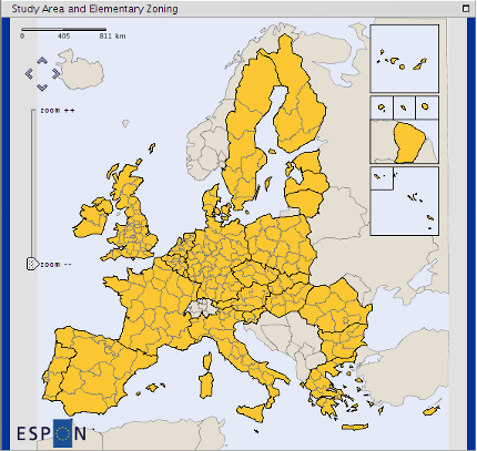
eu31nuts2: this template considers the typical ESPON Area with 31 countries, the lowest mesh level is NUTS 2 in its revision 2006 delineation, as shown on Figure 11.6.
Figure 11.6. EU 31 NUTS 2 study area geometry template overview
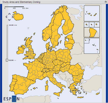
Delineation of the EU 31 NUTS 2 geometry template.
| |
Since version 1.0.2 of the application, the eu27nuts2, eu27nuts3 and eu31nuts2 templates embed a layer that allows to display the main cities over the maps. See Section 6.2 for more details about this service. |
On clicking the name of the chosen template, the user is redirected to the "Input data" page described in Stocks input next chapter.
| |
For your information, the list of units names is given in the appendix Annex: templates units names |
Table of Contents
Once the user has chosen a structure template, he/she is invited to submit his stocks for the study area. Figure 12.2 shows the form page where he/she can:
download the data template example for the selected structure;
upload his/her own statistics and relevant ratios as described in Section 12.1
Figure 12.2. Upload data page
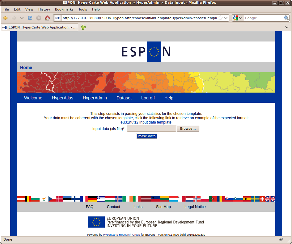
On this page, the user can both download an example and upload his/her own spreadsheet file providing the stocks values for the dataset he/she wants to generate.
Cliking the "Parse data" button triggers the upload of the input data file to the server then its parsing.
| |
Depending on the size of the uploaded file and the number of stocks and ratios to parse, this step may take a while. Please do not click again the submit button as long as the page has not reloaded and displayed any success or failure message. |
In the case when the input data file has been successfully parsed, the user is redirected to the "Build" page, see Build page.
If the input spreadsheet file does not respect the expected format, an error message is displayed at the top of the page.
This section describes the stocks (statistical data) file that ESPON HyperAdmin expects as input.
| |
Please note the following requirements for the input data file:
|
Following sections describe the expected format (sheets, columns and possible values) for the version 2 of this data.xls file.
Table 12.1 provides an example for this mandatory sheet in the data v2 input xls file.
| VERSION | TIME_ENABLED |
|---|---|
| 2 | TRUE |
This sheet aims at identifying the version of the format of this data file. Currently (2010-2011), only the value 2 is possible for the VERSION column.
The expected value for the TIME_ENABLED column is a boolean: only TRUE or FALSE values are possible:
The TRUE value shows that values are available for the sames labels of indicators at several dates: for example, the population in 2000, the population in 2002.
The FALSE value shows that each indicator is given for a single date.
Table 12.2 provides an example for this mandatory sheet in the data v2 input xls file.
| UT_ID | pop2000 | pop2002 | area2000 | gdp2000 | gdp2002 |
|---|---|---|---|---|---|
| AT111 | 1 | 15 | 2 | 7 | 10 |
| AT112 | 3 | 16 | 4 | 8 | 11 |
| AT113 | 5 | 17 | 6 | 9 | 12 |
This sheet must provide at least three columns: UT_ID then at least two indicators identifiers (in HyperAtlas, there must be at least one numerator stock
and one denominator stock). The Table 12.2 shows five indicators identifiers: pop2000, pop2002, area2000,
gdp2000 and gdp2002. These identifiers must be described in the StockInfo sheet (see Section 12.1.8).
The UT_ID column must provide the list of territorial units at the lowest rank (example, at NUTS 3 level) of the dataset. The units are referenced by their
identifiers that must match the given values in the associated structure.xls input file.
Then, each other cell provides a value for the given indicator column at the given unit row. For example in Table 12.2, 17 is the value for pop2002 indicator in AT113 territorial unit.
| |
Each cell must be valuated. Missing values are not accepted here. |
Table 12.3 provides an example for this optional sheet in the data v2 input xls file.
| DEFAULT_NUM | DEFAULT_DEN |
|---|---|
| pop | area |
This sheet aims at providing a default indicator to be selected in HyperAtlas at startup for the denominator and for the numerator combo boxes. Expected values for both columns are valid indicators identifiers that must match two of those defined in the StockInfo sheet (see Section 12.1.8).
Table 12.4 provides an example for this mandatory sheet in the data v2 input xls file.
| LABEL_ID | LANG_CODE | NAME | DESC |
|---|---|---|---|
| 1 | EN | Total population | Total population in thousands |
| 1 | FR | Population totale | Population totale en milliers |
| 2 | EN | Area | Total area |
| 2 | FR | Superficie | Superficie totale |
| 3 | EN | GDP | Gross domestic product |
| 3 | FR | PIB | Produit intérieur brut |
| 4 | EN | GDP/Inhabitant | Gross domestic product per inhabitant |
| 4 | FR | PIB/Hab | PIB par habitant |
| 5 | EN | Density | Density of population |
| 5 | FR | Densité | Densité de population |
This sheet aims at providing the internationalized names and descriptions for the indicators and predefined ratios. The LABEL_ID and LANG_CODE
provides indexes for this table: for a given label identifier there may be several available translations. Thus, the LABEL_ID = 1 is available in english (LANG_CODE = EN) and french
(LANG_CODE = FR) languages. In the StockInfo sheet, each indicator reference a label identifier. As several indicators may
be similarly named and described (when an indicator is valuated for several dates), these labels have been exported here.
| |
The language identifier code must be a valid ISO Language Code. These codes are the lower-case, two-letter codes as defined by ISO-639. Nevertheless, the parser supports upper-cases. You can find a full list of these codes at a number of sites, such as: http://www.ics.uci.edu/pub/ietf/http/related/iso639.txt (2011-03-16). |
Note that values in the LABEL_ID column may be referenced from the StockInfo sheet (see Section 12.1.8)
and from the RatioStock sheet (see Section 12.1.7).
Table 12.5 provides an example for this optional sheet in the data v2 input xls file.
| UT_ID | STOCK_ID | PROVIDER_ID |
|---|---|---|
| AT111 | pop2000 | 1 |
| AT112 | pop2000 | 2 |
| area | 2 | |
| pop2002 | 1 |
This draft sheet aims at providing some basic metadata information for an indicator relatively or not to a territorial unit. Currently, only the source of data may be given as metadata.
For example in Table 12.5, the values of the pop2000 indicator identifier were retrieved from different sources for
regions AT111 and AT112. On the contrary, all values for the area indicator, whatever the unit is,
were provided by the same source. Idem for the pop2002 indicator.
The values in the PROVIDER_ID column must match the identifiers that are given in the Provider sheet (see Table 12.6).
Likewise, the values in the STOCK_ID column must match the identifiers that are defined in the StockInfo sheet (see Table 12.8).
Table 12.6 provides an example for this optional sheet in the data v2 input xls file.
| PROVIDER_ID | NAME | CONTACT | URL |
|---|---|---|---|
| 1 | Eurostat | toto@eurostat.eu | http://www.eurostat.eu |
| 2 | INSEE | tata@insee.fr | http://www.insee.fr |
This sheet aims at providing the list of data providers. Their different ids are referenced from the Metadata sheet.
Table 12.7 provides an example for this optional sheet in the data v2 input xls file.
| RATIO_ID | LABEL_ID | NUM_ID | DEN_ID | VALIDITY_START | VALIDITY_END |
|---|---|---|---|---|---|
| 1 | 4 | gdp2000 | pop2000 | 2000 | 2000 |
| 2 | 4 | gdp2002 | pop2002 | 2002 | 2002 |
| 3 | 5 | pop2000 | area2000 | 2000 | 2000 |
| 4 | 5 | pop2002 | area2000 | 2002 | 2002 |
This sheet aims at defining relevant ratios for the HyperAtlas "ratio" combo box parameter. Table 12.7 shows the example of two such predefined ratios, each of them for two different dates:
the GDP/Inhabitant:
in 2000 (second line)
in 2002 (third line)
The density of population:
in 2000 (fourth line)
in 2002 (fifth line)
Each value in the RATIO_ID column must be unique. Doublons will overwrite the previous found value.
Note that the LABEL_ID references the sames labels for the given pairs of numerator/denominator at different dates (4 for lines 2 and 3, 5 for lines 4 and 5).
These labels identifiers must be set in theLabel sheet (see Section 12.1.4).
The values in the NUM_ID column and the values in the DEN_ID column must match the identifiers of indicators
that are defined in the StockInfo sheet (see Section 12.1.8).
The values in the VALIDITY_START column will only be considered if the value of the TIME_ENABLED column in the About sheet is TRUE (see Section 12.1.1).
Then, one relevant ratio can be chosen in HyperAtlas for different dates.
Identically for the values in the VALIDITY_END column. Though VALIDITY_START and VALIDITY_END
columns are designed to handle time intervals, setting the same value in both columns makes the ratio associated to a timestamp.
Table 12.8 provides an example for this mandatory sheet in the data v2 input xls file.
| STOCK_ID | LABEL_ID | MEASURE_UNIT | VALIDITY_START | VALIDITY_END | VISIBLE_FLAG |
|---|---|---|---|---|---|
| pop2000 | 1 | *1000 | 2000 | 2000 | TRUE |
| pop2002 | 1 | *1000 | 2002 | 2002 | TRUE |
| area2000 | 2 | km2 | 2000 | 2000 | TRUE |
| gdp2000 | 3 | euros | 2000 | 2000 | TRUE |
| gdp2002 | 3 | euros | 2002 | 2002 | TRUE |
This sheet mainly aims at providing the identifiers of the indicators of the dataset. Here are a short description for each column of this sheet:
STOCK_ID: each value in this column must be unique. Any doublon will overwrite the previous found identical value. This column lists the identifiers of the indicators that are referenced in the other sheets. Note that several indicators may be associated to the same label (lines 2 and 3 for example), though they exist to distinguish the values of the population in 2000 and 2002.LABEL_ID: each value in this column must reference an identifier defined in the Label sheet (see Section 12.1.4).MEASURE_UNIT: simply provides the unit of measure for this indicator.VALIDITY_START: shows the start date of validity for this indicator. This field will only be considerated if the value of theTIME_ENABLEDcolumn in the About sheet isTRUE(see Section 12.1.1 and Important note about expected date format).VALIDITY_END: shows the end date of validity for this indicator.VALIDITY_STARTandVALIDITY_ENDfields are able to manage time intervals, but they can be used to associate a timestamp to the current stock: just write the same value in both cells (please see Important note about expected date format).VISIBLE: this field acts like a flag, a boolean is expected for the values of this column. ATRUEvalue shows that this indicator will be available in the numerator and in the denominator combo boxes of HyperAtlas parameters panel. AFALSEvalue may be usefull to define relevant ratios whose indicators have no reason to be available in the numerator and denominator combo boxes. For example, the life expectancy pre-defined ratio considers indicators that have no sense out of this compute.
Once the user has submitted a well-formed spreadhseet file including his/her stocks for the chosen geometry at step 1, he/she is redirected to the "Build" page, see Figure 13.1. He/she is invited here to enter a name and a description for the dataset hyp file he/she is about to generate. These fields are mandatory.
Figure 13.1. Dataset information form
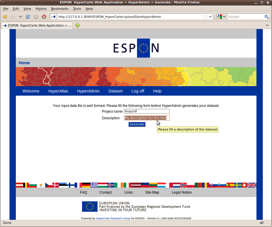
The stock data file is well-formed. Enter a name and a description for the dataset.
| |
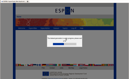
Depending on the wideness of the dataset (number of stocks/geometries/zonings, etc.), this step may take a while. While building the dataset, a progress bar appears after a few seconds in the foreground of the window, the backgound page functionnalities are disabed:
Please do not click the submit button as long as the page has not completly reloaded and displayed a success or failure message. |
If the generation of the hyp file is successfull, the user is redirected to a success page where he/she can download his/her new dataset. Else, an error message is displayed on this "build" page.
In case of success (Figure 13.2), the ouput build logs are summarized and displayed on the page.
In order to avoid overwriting, note that the generated hyp filename follows a date pattern: yyyyMMddhhmmss
(year month date hour minutes seconds). On clicking the link showing the name of the generated dataset, the user is invited to save the file
to his/her disk, of course he/she can rename the hyp file at his/her convenience.
| |
The use of Microsoft Internet Explorer browser may disturb users when clicking the link by opening an ununderstanble page showing the content
of the binary |
Figure 13.2. Successfull build
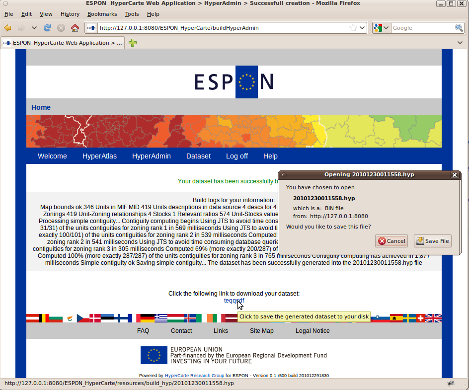
Clicking the link at the bottom of the page invites the user to download his/her generated dataset as an hyp file.
Table of Contents
This section deals with the problems that may occurre when using the described tools in this document.
Below Known bugs section proposes a non-exhaustive list of problems that can be worked around when using the ESPON HyperAtlas software.
Like most of Java applets, the ESPON HyperAtlas software displays logs messages to the "Java Console". This window is not enabled by default on most of standard browsers. If ESPON HyperAtlas does not behave as expected and described in this user's manual, first enable this Java Console. Note that the display of the Java console depends on your operating system and on your Web browser. Please consult the following links (last visit: 20101228):
Windows users: How do I enable and view the Java Console?;
Mac OS X users: Java Frequently Asked Questions
RedHat and Suse Linux users: How do I enable and view the Java Console for Linux?.
For problems that might happen when browsing the pages of the ESPON HyperCarte Web Application, a custom page has been created in order to trace some information. Please copy paste the page and send it to the administrator with as many details on how it happened as possible.
| |
In order to improve the application, thanks in advance for your cooperation, please report bugs! As far as possible, complete your message with eventual output logs, information about your environment, the version of the application, etc. For any comment question or suggestion, please contact the manager. |
ESPON HyperAtlas sometimes seems frozen as nothing happens when changing a parameter. Most of the time, your java console will display the log message shown on Figure A.1.
A simple action allows to workaround this bug: simply resize your window!
Figure A.1. Java console: stroke shape error
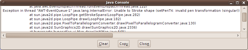
Displayed log message when the maps of HyperAtlas seem frozen.
The deviations maps may sometimes appear "all in grey"... Just click the deviation context combo box in the parameters panel in order that HyperAtlas takes into account the changes of references.
After several analysis with several datasets, multiple messages boxes may appear. As a Java Applet is loaded in memory for a whole browser session, multiple instances may cause this problem.
The simplest thing to workaround this disturbing behaviour is to close your browser, then restart it.
This bug should be fixed in a next iteration.
Table of Contents
For both available ESPON HyperAdmin templates (see Stocks input), this appendix provides the list of names for all units at lowest level of the zoning hierarchy.
"UT_ID","Language_ID","UT_NAME"

"AT11","DE","BURGENLAND (A)"
"AT12","DE","NIEDERÖSTERREICH"
"AT13","DE","WIEN"
"AT21","DE","KÄRNTEN"
"AT22","DE","STEIERMARK"
"AT31","DE","OBERÖSTERREICH"
"AT32","DE","SALZBURG"
"AT33","DE","TIROL"
"AT34","DE","VORARLBERG"
"BE10","FR","RÉGION DE BRUXELLES-CAPITALE/BRUSSELS HOOFDSTEDELIJK GEWEST"
"BE21","FR","PROV, ANTWERPEN"
"BE22","FR","PROV, LIMBURG (B)"
"BE23","FR","PROV, OOST-VLAANDEREN"
"BE24","FR","PROV, VLAAMS BRABANT"
"BE25","FR","PROV, WEST-VLAANDEREN"
"BE31","FR","PROV, BRABANT WALLON"
"BE32","FR","PROV, HAINAUT"
"BE33","FR","PROV, LIÈGE"
"BE34","FR","PROV, LUXEMBOURG (B)"
"BE35","FR","PROV, NAMUR"
"BG31","EN","SEVEROZAPADEN"
"BG32","EN","SEVEREN TSENTRALEN"
"BG33","EN","SEVEROIZTOCHEN"
"BG34","EN","YUGOIZTOCHEN"
"BG41","EN","YUGOZAPADEN"
"BG42","EN","YUZHEN TSENTRALEN"
"CH01","FR","RÉGION LÉMANIQUE"
"CH02","FR","ESPACE MITTELLAND"
"CH03","FR","NORDWESTSCHWEIZ"
"CH04","FR","ZÜRICH"
"CH05","FR","OSTSCHWEIZ"
"CH06","FR","ZENTRALSCHWEIZ"
"CH07","FR","TICINO"
"CY00","EN","CYPRUS"
"CZ01","CS","PRAHA"
"CZ02","CS","STREDNÍ CECHY"
"CZ03","CS","JIHOZÁPAD"
"CZ04","CS","SEVEROZÁPAD"
"CZ05","CS","SEVEROVÝCHOD"
"CZ06","CS","JIHOVÝCHOD"
"CZ07","CS","STREDNÍ MORAVA"
"CZ08","CS","MORAVSKOSLEZSKO"
"DE11","DE","STUTTGART"
"DE12","DE","KARLSRUHE"
"DE13","DE","FREIBURG"
"DE14","DE","TÜBINGEN"
"DE21","DE","OBERBAYERN"
"DE22","DE","NIEDERBAYERN"
"DE23","DE","OBERPFALZ"
"DE24","DE","OBERFRANKEN"
"DE25","DE","MITTELFRANKEN"
"DE26","DE","UNTERFRANKEN"
"DE27","DE","SCHWABEN"
"DE30","DE","BERLIN"
"DE41","DE","BRANDENBURG - NORDOST"
"DE42","DE","BRANDENBURG - SÜDWEST"
"DE50","DE","BREMEN"
"DE60","DE","HAMBURG"
"DE71","DE","DARMSTADT"
"DE72","DE","GIEßEN"
"DE73","DE","KASSEL"
"DE80","DE","MECKLENBURG-VORPOMMERN"
"DE91","DE","BRAUNSCHWEIG"
"DE92","DE","HANNOVER"
"DE93","DE","LÜNEBURG"
"DE94","DE","WESER-EMS"
"DEA1","DE","DÜSSELDORF"
"DEA2","DE","KÖLN"
"DEA3","DE","MÜNSTER"
"DEA4","DE","DETMOLD"
"DEA5","DE","ARNSBERG"
"DEB1","DE","KOBLENZ"
"DEB2","DE","TRIER"
"DEB3","DE","RHEINHESSEN-PFALZ"
"DEC0","DE","SAARLAND"
"DED1","DE","CHEMNITZ"
"DED2","DE","DRESDEN"
"DED3","DE","LEIPZIG"
"DEE0","DE","SACHSEN-ANHALT"
"DEF0","DE","SCHLESWIG-HOLSTEIN"
"DEG0","DE","THÜRINGEN"
"DK01","DA","HOVEDSTADEN"
"DK02","DA","SJÆLLAND"
"DK03","DA","SYDDANMARK"
"DK04","DA","MIDTJYLLAND"
"DK05","DA","NORDJYLLAND"
"EE00","ET","ESTONIA"
"ES11","ES","GALICIA"
"ES12","ES","PRINCIPADO DE ASTURIAS"
"ES13","ES","CANTABRIA"
"ES21","ES","PAIS VASCO"
"ES22","ES","COMUNIDAD FORAL DE NAVARRA"
"ES23","ES","LA RIOJA"
"ES24","ES","ARAGÓN"
"ES30","ES","COMUNIDAD DE MADRID"
"ES41","ES","CASTILLA Y LEÓN"
"ES42","ES","CASTILLA-LA MANCHA"
"ES43","ES","EXTREMADURA"
"ES51","ES","CATALUÑA"
"ES52","ES","COMUNIDAD VALENCIANA"
"ES53","ES","ILLES BALEARS"
"ES61","ES","ANDALUCIA"
"ES62","ES","REGIÓN DE MURCIA"
"ES63","ES","CIUDAD AUTÓNOMA DE CEUTA (ES)"
"ES64","ES","CIUDAD AUTÓNOMA DE MELILLA (ES)"
"ES70","ES","CANARIAS (ES)"
"FI13","FI","ITÄ-SUOMI"
"FI18","FI","ETELÄ-SUOMI"
"FI19","FI","LÄNSI-SUOMI"
"FI1A","FI","POHJOIS-SUOMI"
"FI20","FI","ÅLAND"
"FR10","FR","ÎLE DE FRANCE"
"FR21","FR","CHAMPAGNE-ARDENNE"
"FR22","FR","PICARDIE"
"FR23","FR","HAUTE-NORMANDIE"
"FR24","FR","CENTRE"
"FR25","FR","BASSE-NORMANDIE"
"FR26","FR","BOURGOGNE"
"FR30","FR","NORD - PAS-DE-CALAIS"
"FR41","FR","LORRAINE"
"FR42","FR","ALSACE"
"FR43","FR","FRANCHE-COMTÉ"
"FR51","FR","PAYS DE LA LOIRE"
"FR52","FR","BRETAGNE"
"FR53","FR","POITOU-CHARENTES"
"FR61","FR","AQUITAINE"
"FR62","FR","MIDI-PYRÉNÉES"
"FR63","FR","LIMOUSIN"
"FR71","FR","RHÔNE-ALPES"
"FR72","FR","AUVERGNE"
"FR81","FR","LANGUEDOC-ROUSSILLON"
"FR82","FR","PROVENCE-ALPES-CÔTE D'AZUR"
"FR83","FR","CORSE"
"FR91","FR","GUADELOUPE (FR)"
"FR92","FR","MARTINIQUE (FR)"
"FR93","FR","GUYANE (FR)"
"FR94","FR","REUNION (FR)"
"GR11","EL","ANATOLIKI MAKEDONIA, THRAKI"
"GR12","EL","KENTRIKI MAKEDONIA"
"GR13","EL","DYTIKI MAKEDONIA"
"GR14","EL","THESSALIA"
"GR21","EL","IPEIROS"
"GR22","EL","IONIA NISIA"
"GR23","EL","DYTIKI ELLADA"
"GR24","EL","STEREA ELLADA"
"GR25","EL","PELOPONNISOS"
"GR30","EL","ATTIKI"
"GR41","EL","VOREIO AIGAIO"
"GR42","EL","NOTIO AIGAIO"
"GR43","EL","KRITI"
"HU10","HU","KÖZÉP-MAGYARORSZÁG"
"HU21","HU","KÖZÉP-DUNÁNTÚL"
"HU22","HU","NYUGAT-DUNÁNTÚL"
"HU23","HU","DÉL-DUNÁNTÚL"
"HU31","HU","ÉSZAK-MAGYARORSZÁG"
"HU32","HU","ÉSZAK-ALFÖLD"
"HU33","HU","DÉL-ALFÖLD"
"IE01","EN","BORDER, MIDLANDS AND WESTERN"
"IE02","EN","SOUTHERN AND EASTERN"
"IS00","EN","ICELAND"
"ITC1","IT","PIEMONTE"
"ITC2","IT","VALLE D'AOSTA/VALLÉE D'AOSTE"
"ITC3","IT","LIGURIA"
"ITC4","IT","LOMBARDIA"
"ITD1","IT","PROVINCIA AUTONOMA BOLZANO-BOZEN"
"ITD2","IT","PROVINCIA AUTONOMA TRENTO"
"ITD3","IT","VENETO"
"ITD4","IT","FRIULI-VENEZIA GIULIA"
"ITD5","IT","EMILIA-ROMAGNA"
"ITE1","IT","TOSCANA"
"ITE2","IT","UMBRIA"
"ITE3","IT","MARCHE"
"ITE4","IT","LAZIO"
"ITF1","IT","ABRUZZO"
"ITF2","IT","MOLISE"
"ITF3","IT","CAMPANIA"
"ITF4","IT","PUGLIA"
"ITF5","IT","BASILICATA"
"ITF6","IT","CALABRIA"
"ITG1","IT","SICILIA"
"ITG2","IT","SARDEGNA"
"LI00","EN","LIECHTENSTEIN"
"LT00","LT","LITHUANIA"
"LU00","EN","LUXEMBOURG (GRAND-DUCHÉ)"
"LV00","LV","LATVIA"
"MT00","EN","MALTA"
"NL11","NL","GRONINGEN"
"NL12","NL","FRIESLAND (NL)"
"NL13","NL","DRENTHE"
"NL21","NL","OVERIJSSEL"
"NL22","NL","GELDERLAND"
"NL23","NL","FLEVOLAND"
"NL31","NL","UTRECHT"
"NL32","NL","NOORD-HOLLAND"
"NL33","NL","ZUID-HOLLAND"
"NL34","NL","ZEELAND"
"NL41","NL","NOORD-BRABANT"
"NL42","NL","LIMBURG (NL)"
"NO01","NO","OSLO OG AKERSHUS"
"NO02","NO","HEDMARK OG OPPLAND"
"NO03","NO","SØR-ØSTLANDET"
"NO04","NO","AGDER OG ROGALAND"
"NO05","NO","VESTLANDET"
"NO06","NO","TRØNDELAG"
"NO07","NO","NORD-NORGE"
"PL11","PL","LÓDZKIE"
"PL12","PL","MAZOWIECKIE"
"PL21","PL","MALOPOLSKIE"
"PL22","PL","SLASKIE"
"PL31","PL","LUBELSKIE"
"PL32","PL","PODKARPACKIE"
"PL33","PL","SWIETOKRZYSKIE"
"PL34","PL","PODLASKIE"
"PL41","PL","WIELKOPOLSKIE"
"PL42","PL","ZACHODNIOPOMORSKIE"
"PL43","PL","LUBUSKIE"
"PL51","PL","DOLNOSLASKIE"
"PL52","PL","OPOLSKIE"
"PL61","PL","KUJAWSKO-POMORSKIE"
"PL62","PL","WARMINSKO-MAZURSKIE"
"PL63","PL","POMORSKIE"
"PT11","PT","NORTE"
"PT15","PT","ALGARVE"
"PT16","PT","CENTRO (PT)"
"PT17","PT","LISBOA"
"PT18","PT","ALENTEJO"
"PT20","PT","REGIÃO AUTÓNOMA DOS AÇORES (PT)"
"PT30","PT","REGIÃO AUTÓNOMA DA MADEIRA (PT)"
"RO11","EN","NORD-VEST"
"RO12","EN","CENTRU"
"RO21","EN","NORD-EST"
"RO22","EN","SUD-EST"
"RO31","EN","SUD - MUNTENIA"
"RO32","EN","BUCURESTI - ILFOV"
"RO41","EN","SUD-VEST OLTENIA"
"RO42","EN","VEST"
"SE11","SV","STOCKHOLM"
"SE12","SV","ÖSTRA MELLANSVERIGE"
"SE21","SV","SMÅLAND MED ÖARNA"
"SE22","SV","SYDSVERIGE"
"SE23","SV","VÄSTSVERIGE"
"SE31","SV","NORRA MELLANSVERIGE"
"SE32","SV","MELLERSTA NORRLAND"
"SE33","SV","ÖVRE NORRLAND"
"SI01","EN","VZHODNA SLOVENIJA"
"SI02","EN","ZAHODNA SLOVENIJA"
"SK01","SK","BRATISLAVSKÝ KRAJ"
"SK02","SK","ZÁPADNÉ SLOVENSKO"
"SK03","SK","STREDNÉ SLOVENSKO"
"SK04","SK","VÝCHODNÉ SLOVENSKO"
"UKC1","EN","TEES VALLEY AND DURHAM"
"UKC2","EN","NORTHUMBERLAND, TYNE AND WEAR"
"UKD1","EN","CUMBRIA"
"UKD2","EN","CHESHIRE"
"UKD3","EN","GREATER MANCHESTER"
"UKD4","EN","LANCASHIRE"
"UKD5","EN","MERSEYSIDE"
"UKE1","EN","EAST YORKSHIRE AND NORTHERN LINCOLNSHIRE"
"UKE2","EN","NORTH YORKSHIRE"
"UKE3","EN","SOUTH YORKSHIRE"
"UKE4","EN","WEST YORKSHIRE"
"UKF1","EN","DERBYSHIRE AND NOTTINGHAMSHIRE"
"UKF2","EN","LEICESTERSHIRE, RUTLAND AND NORTHANTS"
"UKF3","EN","LINCOLNSHIRE"
"UKG1","EN","HEREFORDSHIRE, WORCESTERSHIRE AND WARKS"
"UKG2","EN","SHROPSHIRE AND STAFFORDSHIRE"
"UKG3","EN","WEST MIDLANDS"
"UKH1","EN","EAST ANGLIA"
"UKH2","EN","BEDFORDSHIRE, HERTFORDSHIRE"
"UKH3","EN","ESSEX"
"UKI1","EN","INNER LONDON"
"UKI2","EN","OUTER LONDON"
"UKJ1","EN","BERKSHIRE, BUCKS AND OXFORDSHIRE"
"UKJ2","EN","SURREY, EAST AND WEST SUSSEX"
"UKJ3","EN","HAMPSHIRE AND ISLE OF WIGHT"
"UKJ4","EN","KENT"
"UKK1","EN","GLOUCESTERSHIRE, WILTSHIRE AND BRISTOL/BATH AREA"
"UKK2","EN","DORSET AND SOMERSET"
"UKK3","EN","CORNWALL AND ISLES OF SCILLY"
"UKK4","EN","DEVON"
"UKL1","EN","WEST WALES AND THE VALLEYS"
"UKL2","EN","EAST WALES"
"UKM2","EN","EASTERN SCOTLAND"
"UKM3","EN","SOUTH WESTERN SCOTLAND"
"UKM5","EN","NORTH EASTERN SCOTLAND"
"UKM6","EN","HIGHLANDS AND ISLANDS"
"UKN0","EN","NORTHERN IRELAND"
"UT_ID","Language_ID","UT_NAME"

"W11111","EN","Denmark"
"W11112","EN","Finland"
"W11113","EN","United Kingdom"
"W11115","EN","Ireland"
"W11116","EN","Iceland"
"W11117","EN","Norway"
"W11118","EN","Sweden"
"W11121","EN","Austria"
"W11122","EN","Belgium"
"W11123","EN","Switzerland"
"W11124","EN","Germany"
"W11125","EN","France"
"W11126","EN","Luxembourg"
"W11127","EN","Netherlands"
"W11131","EN","Spain"
"W11132","EN","Greece"
"W11133","EN","Italy"
"W11134","EN","Portugal"
"W11135","EN","Cyprus"
"W11136","EN","Malta"
"W11211","EN","Czech Republic"
"W11212","EN","Estonia"
"W11213","EN","Hungary"
"W11214","EN","Lithuania"
"W11215","EN","Latvia"
"W11216","EN","Poland"
"W11217","EN","Slovakia"
"W11218","EN","Slovenia"
"W11221","EN","Albania"
"W11222","EN","Bulgaria"
"W11223","EN","Croatia"
"W11224","EN","Macedonia, TFYR"
"W11225","EN","Romania"
"W11226","EN","Serbia/Montenegro"
"W11227","EN","Bosnia and Herzegovina"
"W11228","EN","Turkey"
"W11231","EN","Armenia"
"W11232","EN","Azerbaijan"
"W11233","EN","Belarus"
"W11234","EN","Georgia"
"W11235","EN","Moldova, Rep. of"
"W11236","EN","Ukraine"
"W11240","EN","Russian Federation"
"W12111","EN","Algeria"
"W12112","EN","Western Sahara"
"W12113","EN","Libyan Arab Jamahiriya"
"W12114","EN","Morocco"
"W12115","EN","Tunisia"
"W12121","EN","Egypt"
"W12122","EN","Israel"
"W12123","EN","Jordan"
"W12124","EN","Lebanon"
"W12125","EN","Syrian Arab Republic"
"W12126","EN","Occupied Palestinian Territories"
"W12211","EN","Kazakhstan"
"W12214","EN","Turkmenistan"
"W12215","EN","Uzbekistan"
"W12221","EN","United Arab Emirates"
"W12222","EN","Bahrain"
"W12223","EN","Iran, Islamic Rep. of"
"W12224","EN","Iraq"
"W12225","EN","Kuwait"
"W12226","EN","Oman"
"W12227","EN","Qatar"
"W12228","EN","Saudi Arabia"
"W12229","EN","Yemen"
"W13126","EN","Chad"
"W13213","EN","Eritrea"
"W13217","EN","Sudan"
"W13329","EN","Mali"
"W1332A","EN","Mauritania"
"W1332B","EN","Niger"
"W1332C","EN","Senegal"
Find here an alphabetical arrangement of most often used acronyms in this document:
Table of Contents
- Deviation
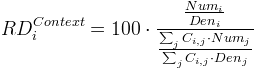
The relative deviation of a given region (i) to a context is defined by equation Figure D.1. The relative deviation depends on the chosen context (general, medium or local), it shows the gap between the value of the unit and the average value of the context. The deviation is expressed in a percentage of the context average value (100 is the pivot).
Figure D.1. Mathematical formula of the relative deviation
This figure shows a general formula to compute the relative deviation
RDof a territorial unit i for the chosen contextContext. Needed variables are:Numx is the value of the indicator chosen as the Numerator parameter for the territorial unitx.Denx is the value of the indicator chosen as the Denominator parameter for the territorial unitx.Cij is a boolean whose value depends on the chosen context:General context:
Cij=1 if the current territorial unitjis included in the reference area,Cij=0 in other cases. For example, if the reference area is EU-15,Cij takes the value 1 for regions of EU-15 and the value 0 for regions of the candidate countries.Territorial context:
Cij shows if two regionsiandjbelong or not to the same area. In the case when the medium context considers the state level,Cij takes the value 1 for regions belonging to the same state and the value 0 for regions belonging to different states.Spatial context:
Cij shows the potential level of local interactions between two regionsiandj. The local interaction may be for example defined by a boolean variable which takes the value 1 for contiguous regions and the value 0 for non-contiguous regions. Currently, we have decided that a region is not neighbour to itself (Locii=0) but it is possible to choose the solution where a region is part of its own neighbourhood (Locii=1). Many alternative solutions are possible according to the definition of the neighbourhood criterion (kilometres time, cost, length of common boundary, ...) and to the measure of the potential level of interaction. This parameter may not be a boolean but a continuous probabilistic function between 0 and 1.
See Also General deviation, Spatial deviation, Territorial deviation.
- Elementary unit
The set of elementary units compose (cover) the whole area, and constitute the elementary zoning.
See Also Elementary zoning.
- Elementary zoning
Smallest division of the studied area. Each unit of this zoning is called elementary unit.
See Also Elementary unit.
- General deviation
Deviation when the context of reference is the general area. The reference can be an available study area or a any value chosen by the user.
See Also Deviation.
- Spatial deviation
Deviation when the context of an unit is defined by the set of units that belongs to its neighbourhood (for instance adjacent units), contiguous regions by default.
See Also Deviation.
- Territorial deviation
Deviation when the context is defined by a territorial unit that belongs to a chosen higher zoning level which contains the considered unit.
See Also Deviation.
- NUTS (Nomenclature of territorial units for statistics)
Established by EUROSTAT for over 30 years, NUTS is a territorial subdivision system used in Europe "in order to provide a single uniform breakdown of territorial units for the production of regional statistics in the European Union" [1]. The NUTS zoning nomenclature for Europe organizes all units in a hierarchy of levels:
NUTS 0groups administrative units at country level : France, Germany, Spain, Italy, etc.NUTS 1groups administrative units at great region level : ILE DE FRANCE, BASSIN PARISIEN, EST, CENTRE-EST, etc.NUTS 2groups administrative units at region level (Région in France - Länder in Germany - Comunidades autonomas in Spain, regioni in Italy) : ILE DE FRANCE, RHONE-ALPES, PACA, etc.NUTS 3groups administrative units at departement level (Département in France - Kreise in Germany - Provincias in Spain, Provincie in Italy): Essone, Isère, Savoie, etc.NUTS 4andNUTS 5are now deprecated levels that are respectively replaced byLAU 1andLAU 2. LAU acronym stands for Local Administrative Unit.
- Report
HTML document that lists the set of parameters used for analysis (study area, zoning, context for deviation, indicators for numerator and denominator) and the maps which are generated by the application.
- Stock
Social-economic count, like number of deaths on 1999 year, number of births on 1999 year, total population in thousand on 1999 year. Stocks should be valued on each elementary unit. There are also called indicators.
- Study Area
Territorial space on which we will base the analysis. It can be Europe, Cameroun, or France by example. Only one study area can be loaded in the same time by the application.
- Ratio
A ratio between two stocks which are defined and available on the same set of territorial units.
- Workspace
Context of analysis and selected options in the application when working on a study area: zoom level, map mode, etc. It can be exported to an XML file.
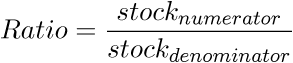
Table of Contents
[1] ESPON. [on line]. http://www.espon.eu/ (last visit: 1.st december 2009).
[2] Appendix J: MapInfo Data Interchange Format. [on line]. http://resource.mapinfo.com/static/files/document/1074660800077/interchange_file.pdf (last visit: 18.th may 2010).
This application is proctected by copyright law
© ESPON, 2013. All rights reserved
Please read the terms and conditions of use carfully.
The ESPON 2013 Programme, by these terms and conditions of use, allows the visitor a non-exclusive and non-transferable right to access to the ESPON 2013 HyperAtlas.The user/visitor is responsible for providing all software and equipment needed to access this service. "User/Visitor" means the company, entity, or individual installing or using the ESPON 2013 HyperAtlas. "Use" means storing, loading, installing, executing, or displaying the ESPON 2013 HyperAtlas and/or its content.
The visitor may use the data included in the ESPON 2013 HyperAtlas for non-profit purposes only, including the production of derivative works for the purpose of illustration for teaching or for another professional or personal use.
No material may be modified, edited or taken out of context whereby its use creates a false or misleading statement or impression of the content of the ESPON 2013 Programme. The user/visitor has no right to sell or redistribute the information included in the ESPON 2013 HyperAtlas.
The source has to be cited as "© ESPON HyperAtlas, 2013".
The ESPON 2013 Programme shall have the right to terminate the user's ability to access this service at any time without notice and also reserves the right to discontinue or modify any of the information contained on this service, or the service, at any time.
The user of the ESPON 2013 HyperAtlas assumes all responsibility and risk for the use of this server and the Internet generally. The ESPON 2013 Programme disclaims all warranties, representations or endorsements, expressed or implied, with regard to the information accessed from, or via, this server or the internet, including, but not limited to, all implied warranties of merchantability, fitness for a particular purpose, or non infringement. In no event shall the ESPON 2013 Programme be liable for any compensatory, special, direct, incidental, indirect, consequential damages, exemplary damages or any damages whatsoever resulting from the use of the data, whether in an action of contract, tort or otherwise, arising out of or in connection with the use or performance of the information on this server or the internet generally or on any other basis.
The ESPON 2013 Programme reserves its exclusive right in its sole discretion to alter, limit or discontinue the site or any materials in any respect. The ESPON 2013 Programme shall have no obligation to take the needs of any visitor into consideration in connection therewith.
The ESPON 2013 HyperAtlas system, software, material and data are protected by copyright and other laws respecting property rights.
The ESPON HyperAtlas Application is owned by the ESPON Programme and developed on the HyperAtlas software. The data and material included in the ESPON 2013 HyperAtlas is a shared property of the ESPON 2013 Programme and the Transnational Project Groups delivering the data/material.
The HyperAtlas software is the property of the Hypercarte Research Group. Code sources of the application ESPON HyperAtlas remain the property of the HyperCarte Research Group. Participants of the HyperCarte Research Group are the LIG-STEAMER and LIG-MESCAL (research teams which both belong to the LIG laboratory, UMR CNRS 5217), the Géographie-cités laboratory (UMR CNRS 8504), and RIATE (UMS CNRS 2414) and their respective supervision research institutes: CNRS, INRIA, Université de Paris 1, Université de Paris 7, Institut National Polytechnique de Grenoble, Université Joseph Fourier and Université Pierre Mendès France.
For any question or demands for assistance regarding the ESPON 2013 HyperAtlas, please contact: <database@espon.eu>.
The use of the ESPON 2013 HyperAtlas is subject to existing laws and legal process. The Terms and Conditions of Use of the ESPON 2013 HyperAtlas shall be governed by the laws of Grand Duchy of Luxembourg. Any dispute arising shall be subject to the personal and exclusive jurisdiction and venue of the Grand Duchy of Luxembourg.
The most relevant laws on this issue are:
Loi du 30 mai 2005 - Protection des données et communications électroniques
Loi du 2 août 2002 - Protection des données
Loi du 18 avril 2001 - Droits d'auteur, les droits voisins et les bases de données
The visitor acknowledges having read these Terms and Conditions agrees to abide by them. The visitor also agrees that the Terms and Conditions supersede all proposals and/or prior agreements, oral and written, and any other communications between the parties.
This document is part of the ESPON HyperCarte Web Application.
This document is expected to be available from the HyperCarte Web Application Help menu item in HTML and PDF formats.
Credits:
For any comment question or suggestion, please visit http://www.espon.eu or contact <manager@espon.eu>.
[1] [on line] GIMP - The GNU Image Manipulation Program (last visit: 2.nd april 2009).
[2] [on line] TEX2PNG Conversion d'une formule LaTeX en image PNG (last visit: 25.th may 2010).
Colophon
This document was generated
2013-07-05 15:23:54 (year-month-date hour:minutes:seconds) from the svn rev 1088 of the docbench project.
Based on DocBook technology [3], this document is written in XML format, sources are validated with DocBook DTD 4.5CR3, then sources are transformed to HTML and PDF formats by using DocBook xslt 1.73.2 stylesheets.
Documents generations were automatized with ant [4], java[5], processors Xalan[6] and FOP [7].
| |
Xslt standard stylesheets are customized in order to get a better image resolution in PDF generated output for admonitions icons: the generated sizes of these icons were turned from 30 to 12 pt. |
[3] [on line] DocBook.org (last visit: november 2009)
[4] [on line] Apache Ant - Welcome. Version 1.7.0. (last visit: 18 november 2009)
[5] [on line] Developer Resources For Java Technology (last visit: 18 november 2009). Version 1.6.0_03-b05.
[6] [on line] Xalan-Java Version 2.7.1 (last visit: 18 november 2009). Version 2.7.1.
[7] [on line] Apache FOP (last visit: 18 november 2009). Version 0.94.